
SLAB-RS, Part 4: The Agent Breaks Its Ceiling with Embeddings
Published:
Part 3 ended at a measured ceiling. Five experiments improved keyword search from nDCG@10 0.2995 to 0.3260, the last improvement was worth two tenths of a percent, and 27 of the 225 test queries still found nothing relevant in their top 10 — because they ask for things using words their answer documents never use. You cannot keyword-match your way out of a vocabulary mismatch.
This is the problem embeddings exist to solve. An embedding turns text into a list of numbers — a vector — placed so that texts with similar meaning end up near each other, even when they share no words. “High-speed aircraft heating” can find a document about “thermal effects at supersonic velocities.”
That is the promise. This article is the story of making it actually work on a production search engine, which took three attempts, one instructive detour, and a lot of discipline about negative results.
The number to beat throughout: 0.3260, the keyword ceiling from Part 3.
Division of labor, as in Part 3: this article covers eight more experiments, and my only intervention among them was proposing learning-to-rank. Everything else — including every accept and reject decision — was the agent’s loop.
Attempt Zero: Test the Plumbing With Fake Vectors
The agent’s first move was not to grab a fancy model. It built the machinery first — a place to store embeddings, a way to search by vector similarity, a way to score the results — and tested it with deliberately meaningless vectors generated from text hashes. A control group.
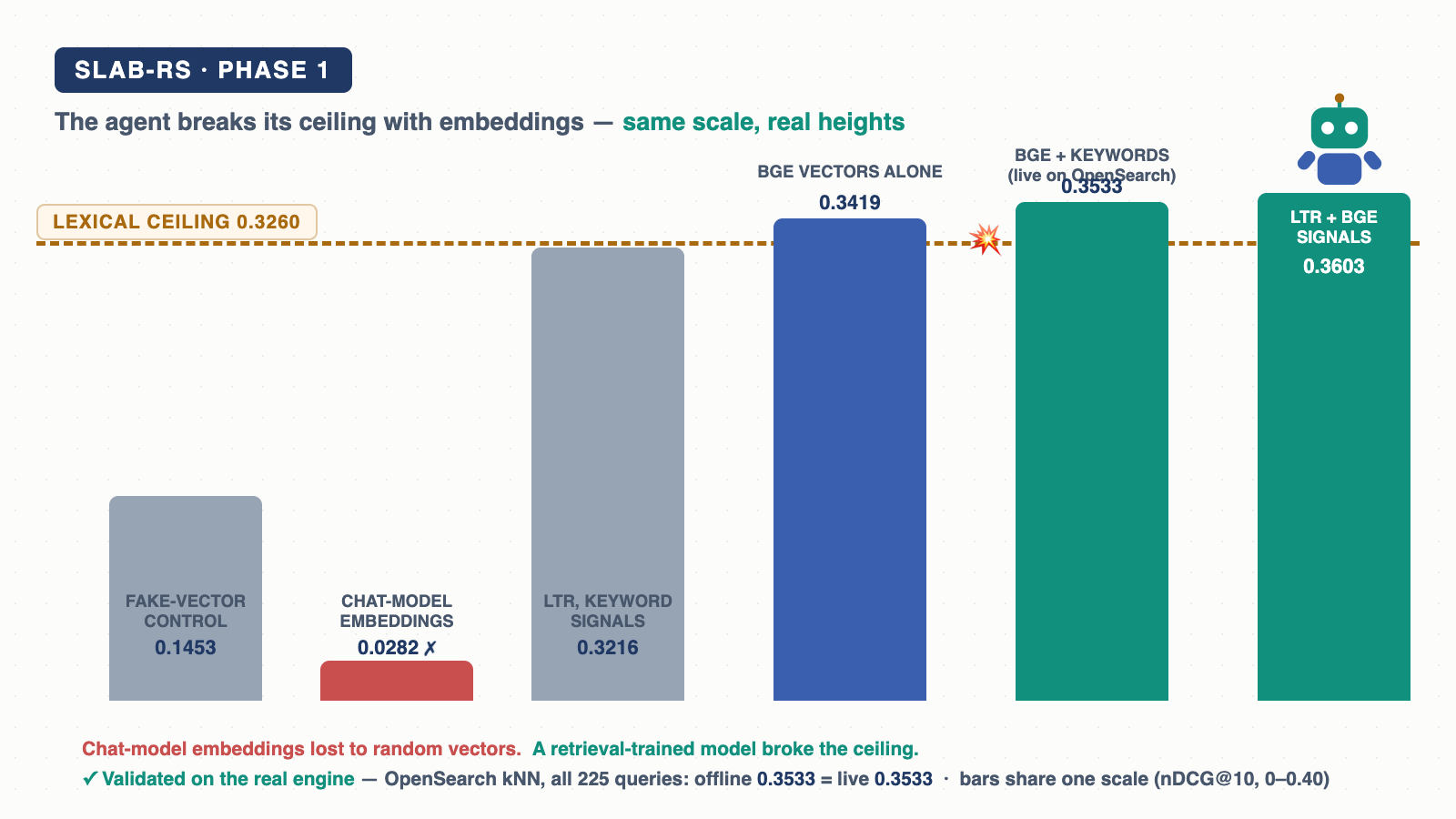
Result: vector-only search scored 0.1453. Mixed with keyword scores, 0.3054. Both well below the keyword ceiling — exactly as they should be, because these vectors carry no meaning. The machinery worked; any future gain would have to come from the model, not the plumbing. Cheap controls first is a habit worth stealing.
Attempt One: Embeddings From a Chat Model Fail, Loudly
Next, real embeddings from a real LLM — a locally-running llama3.1:8b, the kind of model you would chat with, producing 4,096 numbers per document.
Result: vector-only search scored 0.0282.
Not a typo. An 8-billion-parameter language model’s embeddings performed five times worse than the random hash vectors. The lesson is fundamental: what makes embeddings good for search is not the model’s size — it is what the model was trained to do. Chat models are trained to generate text. Nothing in that training pushes “query” and “document that answers it” to be near each other in vector space. Models trained specifically for retrieval do exactly that. “Semantic search” is not one thing.
Blending the chat-model vectors with keyword scores clawed back to 0.3035 — still below the ceiling. Rejected, with all the results kept public. This negative result is what makes the eventual win believable.
The Detour: How Much Better Could Ranking Even Get?
This is where my second — and final — intervention of the phase happened: I proposed trying learning to rank, training a model to re-order results instead of hand-tuning bonuses.
What the agent did with the proposal is the interesting part. Before training anything, it asked a question I wish more teams asked: if we re-ordered what we already retrieve absolutely perfectly, how good would the results be?
The answer: 0.7033 — against an achieved 0.3260. In other words, for most queries the good documents are already being fetched in the top 50; they are just ordered badly. Huge headroom — so the proposal was worth pursuing, and the agent could say why before spending anything on training.
Two trainers were built and tested carefully — with cross-validation, meaning the model is always scored on queries it never saw during training. On a dataset of only 225 queries, skipping that step produces numbers that look great and mean nothing (the classic overfitting trap).
The honest result: with keyword-based signals, the best learned ranker scored 0.3216 — below the ceiling. The training-set scores looked much better (up to 0.3564), and were recorded strictly as “the machinery has capacity” evidence, nothing more. Conclusion at this point: the ranking machinery works, but its input signals carry nothing the keyword ladder didn’t already have.
The Breakthrough: A Model Built for Retrieval
Attempt three used a model trained for exactly this job: BGE (BAAI/bge-base-en-v1.5), a compact open-source retrieval model producing 768 numbers per text.
Everything changed at once:
| Approach | nDCG@10 | vs keyword ceiling (0.3260) |
|---|---|---|
| BGE vectors alone | 0.3419 | +4.9% |
| BGE + keyword scores together | 0.3533 | +8.4% |
| Learned ranker with BGE signals added | 0.3603 | +10.5% |
Three observations worth articles of their own:
- The purpose-built 768-number model beat the 4,096-number chat model by 12× (0.3419 vs 0.0282). Size is not the story. Training objective is the story.
- Vectors plus keywords beat vectors alone. The two approaches fail on different queries, so combining them wins. This matches what most production teams find.
- The learned ranker that failed suddenly worked. Same trainer, same process — but once BGE similarity was added as an input signal, it went from below the ceiling to the best score of the entire phase. A ranking model is only as good as what you feed it.
Making It Production-Shaped
A win in an offline evaluation script is a notebook result, not an architecture. So the embeddings were loaded into a real OpenSearch vector index — a separate one, leaving the public index untouched — and the full 225-query evaluation was re-run live against the actual engine.
The live result matched the offline number exactly: 0.3533. On the comparison scale from Part 3, the live hybrid scored 0.4926 — which finally beats the BM25 result (0.4714) from Ghasemi and Hiemstra’s “BERT meets Cranfield” paper, though their BERT rankers (0.5525–0.5670) remain ahead. That gap is real — and, as I explain below, one I am deliberately not chasing on this dataset.
When the offline and live numbers agree to four decimal places, you can start calling it a candidate architecture.
Shipping Honesty: The 501
Here is an unusual production decision, and my favorite detail of the phase. The public site exposes every architecture milestone as a stable endpoint — baseline, feedback rerank, and BGE. But live BGE search needs the query turned into a vector at request time, and the public API layer has no embedding model running in it yet. The usual demo move is to fake it.
Instead, the BGE endpoint returns an explicit “501 — runtime not enabled” along with the validated evidence, the index name, and the stated next step. The explain page shows it as an honest status card next to the two live architectures, with archived sample results you can replay. A 501 with evidence is a better public artifact than a demo that pretends.
And the BGE hybrid is still — deliberately — not the public default. The same gate that held back every keyword candidate holds here: nothing is promoted until it proves itself on a second dataset (BEIR is the next phase), and until the latency, cost, and runtime pieces are real.
The Full Picture: Sixteen Experiments, Two Human Interventions
The chain for this article, each step reached from the previous one’s evidence:
- The keyword ceiling and the 27 vocabulary-mismatch queries (Part 3) → try embeddings.
- Build the vector machinery first → the fake-vector control (agent) proved the plumbing without a model.
- First real model → chat-model embeddings (agent, rejected — 0.0282).
- My LTR proposal → the agent’s headroom analysis (0.7033 possible), then two learned rankers with keyword signals (agent, both below the ceiling — honest cross-validated scores).
- “The features are the problem, not the machinery” → a retrieval-trained model, BGE (agent) — first to beat the ceiling.
- BGE works offline → BGE signals into the learned ranker (agent) — best score of the phase.
- Offline is not production → live OpenSearch vector index (agent) — the offline number reproduced exactly.
Phase 1 in one table — sixteen experiments across the two articles, four explicit rejections, two human interventions (the paper pointer and the LTR proposal), six days:
| Milestone | nDCG@10 | vs baseline |
|---|---|---|
| BM25 baseline (released, public default) | 0.2995 | — |
| Keyword ceiling: feedback rerank (candidate) | 0.3260 | +8.8% |
| BGE + keywords, live on OpenSearch (candidate) | 0.3533 | +18.0% |
| Learned ranker with BGE signals (cross-validated) | 0.3603 | +20.3% |
Along the way: a boost-clause idea that regressed, a query-expansion idea that regressed, fake vectors that behaved exactly as fake vectors should, chat-model embeddings that failed spectacularly, and a learned ranker that lost twice before the right signals arrived — all preserved as public artifacts, because the rejections are what give the accepted numbers their meaning.
Takeaways
- Run cheap controls before paying for real models — and publish the negative results; they are what make the win believable.
- “Semantic search” is not one thing. The gap between a chat model’s embeddings and a retrieval-trained model’s embeddings was the entire difference between failure and breakthrough.
- Validate vector wins on the production engine, not just offline — and stay suspicious until the numbers agree.
- Ship honesty: an explicit 501 with evidence beats a faked demo, and a promotion gate you actually enforce beats a leaderboard.
Closing Phase 1: Why I Am Not Chasing the Cranfield Leaderboard
To be clear, this is not a victory declaration on Cranfield. The paper’s BERT rankers still score higher, and with enough Cranfield-specific tuning we could probably close more of that gap. But the system now stands on the same state-of-the-art retrieval technology behind modern results — retrieval-tuned dense embeddings, hybrid scoring, learned ranking, all validated on a production engine — and reaching that standard, not topping a leaderboard, was the point.
I am deliberately not spending more time on Cranfield, for two reasons. First, Cranfield is not retail data: each document is flat text, not a product with structured fields like title, brand, color, attributes, and price. Second, whatever more we squeeze out of Cranfield-specific optimization may not transfer — and non-transferable wins are exactly what this project is designed to reject.
Cranfield’s job was different, and it is done: prove the IR fundamentals — a measured baseline, honest evaluation, failure-driven experiments, evidence-gated promotion — before any product-specific tuning. With this article, Phase 1 closes.
Phase 2 is about transferability: the candidates that won here go to BEIR, a benchmark suite spanning many different domains, and only the techniques that prove they generalize beyond aeronautics keep their place in the architecture. That gate decides what travels with us toward real retail product search.