<?xml version="1.0" encoding="utf-8"?><feed xmlns="http://www.w3.org/2005/Atom" ><generator uri="https://jekyllrb.com/" version="3.10.0">Jekyll</generator><link href="https://feroshjacob.github.io/feed.xml" rel="self" type="application/atom+xml" /><link href="https://feroshjacob.github.io/" rel="alternate" type="text/html" /><updated>2026-10-05T15:01:41+00:00</updated><id>https://feroshjacob.github.io/feed.xml</id><title type="html">Ferosh Jacob, Ph.D.</title><subtitle>Ferosh Jacob is a software engineering and AI leader with a Ph.D. in computer science, focused on search, relevance, data science, and practical AI systems.</subtitle><author><name>Ferosh Jacob</name><email>feroshjacob@gmail.com</email><uri>https://feroshjacob.github.io</uri></author><entry><title type="html">Part 4: Providing Affordable SEO for Small Business Using Jev (Part 1)</title><link href="https://feroshjacob.github.io/posts/2026/10/05/modern-software-for-small-businesses-and-nonprofits-part-4-providing-affordable-seo-for-small-business-using-jev-part-1" rel="alternate" type="text/html" title="Part 4: Providing Affordable SEO for Small Business Using Jev (Part 1)" /><published>2026-10-05T00:00:00+00:00</published><updated>2026-10-05T00:00:00+00:00</updated><id>https://feroshjacob.github.io/posts/2026/10/05/modern-software-for-small-businesses-and-nonprofits-part-4-providing-affordable-seo-for-small-business-using-jev-part-1</id><content type="html" xml:base="https://feroshjacob.github.io/posts/2026/10/05/modern-software-for-small-businesses-and-nonprofits-part-4-providing-affordable-seo-for-small-business-using-jev-part-1"><![CDATA[<p class="align-center">
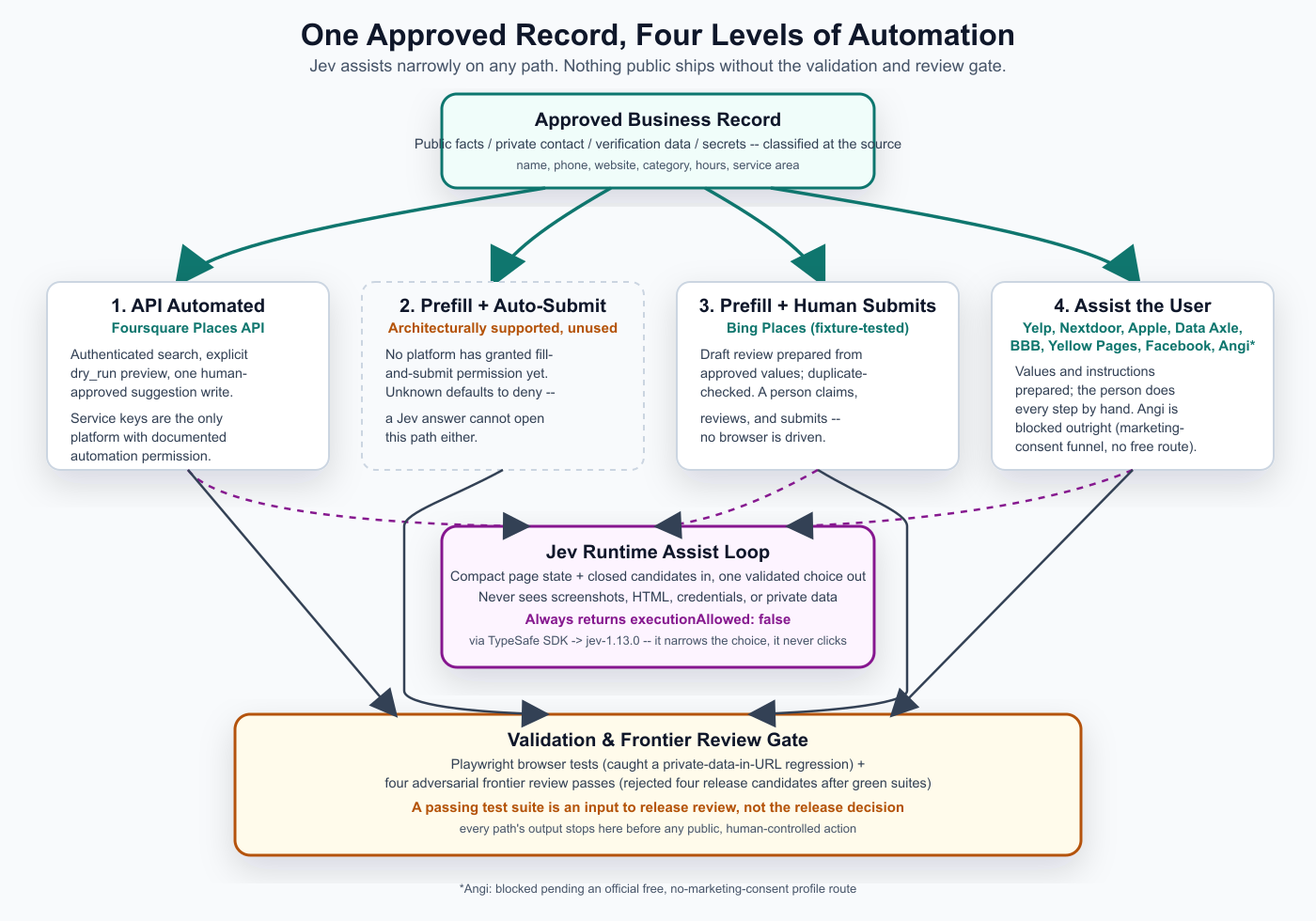
  <img src="/images/modern-software-part4-jev-seo-architecture.png" alt="Diagram: one approved business record feeding four levels of automation -- API automated, prefill with auto-submit (unused), prefill with human submit, and assist-the-user -- with a narrow Jev assist loop and a validation and review gate in front of every path" style="max-width: 100%; height: auto;" />
</p>

<p>This is Part 4 of the <a href="https://feroshjacob.github.io/series/modern-software-small-businesses-nonprofits/">Modern Software for Small Businesses and Nonprofits</a> series, and Part 1 of a new sub-topic inside it: providing affordable SEO for small business, starting with local business-listing profiles, and starting with Jev doing the narrow work it’s actually good at.</p>

<h2 id="the-short-version">The short version</h2>

<p>SEO tools that can manage more than five or six sites at once can easily cost $1,000 a month. For an agency to make a living reselling that, a small business ends up paying several thousand dollars a month — money that is not affordable for most of them. So I’m building a small, human-assisted tool that creates one approved business record once and prepares it for ten listing sites, as an experiment. It is semi-automated on purpose, because the sites themselves don’t all allow the same thing, and I’d rather be honest about that than ship something that gets a client’s listing suspended.</p>

<h2 id="the-problem-seo-pricing-locks-small-business-out-before-it-starts">The problem: SEO pricing locks small business out before it starts</h2>

<p>Here’s the plain fact I keep running into: the popular SEO tools that can manage more than five or six client sites can easily cost $1,000 a month. An agency buying that tooling has to recover it across its client base, and the bill that lands on an individual small business is several thousand dollars a month. That’s not a business decision a solo tea shop or a two-truck pet-waste company gets to make — it’s simply out of reach.</p>

<p>Local listing profiles (Google, Bing, Yelp, Nextdoor, and the rest) are one of the cheapest, highest-leverage pieces of local SEO there is, and they’re exactly the kind of repetitive, multi-site data entry a small agency charges for. So the first experiment in this sub-series is narrow: can one approved record be reused across ten listing platforms without an agency retainer, and without quietly breaking any site’s rules to do it?</p>

<h2 id="what-jev-is-in-plain-terms">What Jev is, in plain terms</h2>

<p>I don’t expect anyone to already know what Jev is, so here it is simply: Jev is an AI model I reach through <a href="https://typesafe.ai">TypeSafe’s</a> official SDK (<a href="https://docs.typesafe.ai">docs.typesafe.ai</a>), and I use it only for narrow, bounded decisions — not for writing code and not for driving a browser.</p>

<p>Jev shows up in exactly one place in the running application: a loopback-only “runtime assist” endpoint. A human supplies compact, visible page state and a closed set of candidate answers; Jev picks among them; the endpoint validates the choice against the candidates it was given and always returns <code class="language-plaintext highlighter-rouge">executionAllowed: false</code>. It cannot navigate, fill a field, upload anything, submit anything, or expand what an adapter is allowed to do.</p>

<h2 id="why-semi-automated-not-fully-automated">Why semi-automated, not fully automated</h2>

<p>Before writing a single adapter, I decided to validate, not assume, what each site’s rules actually say — so here’s what I found, and where I still don’t know.</p>

<p>The common framing is this: some sites simply won’t let a bot click “submit,” and stricter sites won’t let a bot populate the form fields at all. That’s real, but it undersells how granular the actual permission question is. I ended up tracking each platform’s permission on several separate dials — business eligibility, free-profile availability, read/navigate, fill, upload, submit, account/verification requirements, and address visibility — and every one of them defaults to <strong>unknown means deny</strong>. A Jev answer cannot grant a capability; only documented, official evidence can.</p>

<p>What that produced, platform by platform:</p>

<ul>
  <li><strong>Foursquare</strong> documents that service API keys are explicitly intended for internal automation, scripts, and agents — the only platform of the ten with an affirmative automation grant. (<a href="https://docs.foursquare.com/fsq-developers-places/reference/authentication">authentication</a>, <a href="https://docs.foursquare.com/fsq-developers-places/reference/place-search">place search</a>, <a href="https://docs.foursquare.com/fsq-developers-places/reference/places-suggest-place">suggest place</a>)</li>
  <li><strong>Bing Places</strong> documents a free claim/add/update flow and lets an eligible service-area business hide its public address, but nothing in the official help establishes permission to automate its web interface. (<a href="https://www.bing.com/forbusiness/help/modernExperience?setlang=en">Bing for Business help</a>)</li>
  <li><strong>Nextdoor</strong> documents a free Business Page for local, casual-service, and home-service providers, requiring an owner or authorized representative to claim it. (<a href="https://business.nextdoor.com/en-us/getting-started/business-page">Create a Business Page</a>)</li>
  <li><strong>Data Axle</strong> documents a free route for one to ten listings with duplicate matching and verification. (<a href="https://www.data-axle.com/marketing-solutions/local-listings-management/">Local Listings</a>)</li>
  <li><strong>Yelp</strong> documents that claiming a page is free but requires owner or representative verification. (<a href="https://business.yelp.com/resources/articles/creating-a-yelp-page-for-your-brand-new-business/">Creating a Yelp Page</a>)</li>
  <li><strong>BBB</strong> separates a free Business Profile from paid accreditation — the pilot is never allowed to drift into the accreditation funnel. (<a href="https://www.bbb.org/get-listed">Get Listed</a>)</li>
  <li><strong>Angi</strong> is the one I actually blocked: its signup funnel asks for a mobile number and explicitly authorizes marketing calls and texts, and I could not find a free, no-lead-funnel profile route. Until that changes, it’s blocked outright, not “manual.” (<a href="https://signup.angi.com/pro/join">Angi pro join</a>)</li>
  <li><strong>Apple Business</strong>, <strong>Yellow Pages</strong>, and <strong>Facebook Pages</strong> all have a documented free or claimable path, but none of them establish enough about address visibility, eligibility, or current terms to automate anything beyond preparing values for a human.</li>
</ul>

<p>So “semi-automated” isn’t a hedge — it’s the honest description of ten sites that each permit something different, with the default on every undocumented permission set to deny.</p>

<h2 id="the-architecture">The architecture</h2>

<p>The diagram above is the real shape of the system: one approved, source-attributed business record feeds four possible levels of automation, Jev sits in a narrow assist loop that any of those levels can call into but that can never act on its own, and nothing reaches a live platform without passing a validation gate and a second, adversarial review from a stronger model first.</p>

<ol>
  <li><strong>API automated — Foursquare.</strong> The only platform with a documented automation grant. The adapter does an authenticated duplicate search, an explicit <code class="language-plaintext highlighter-rouge">dry_run=true</code> preview, and then one human-approved <code class="language-plaintext highlighter-rouge">dry_run=false</code> suggestion write — never a browser interaction with Foursquare’s business portal.</li>
  <li><strong>Prefill + automated submit.</strong> Architecturally supported by the adapter contract, but currently unused by every one of the ten platforms, because none of them has granted fill-and-submit permission. This is the level where “unknown means deny” actually bites: Jev being confident about a field does not open this path either.</li>
  <li><strong>Prefill + human submits — Bing.</strong> A fixture-tested draft review is prepared from the approved record, checked against known duplicates, and handed to a person to claim, review, and submit. No browser drives Bing’s site.</li>
  <li><strong>Assist the user — the other eight platforms.</strong> Values and instructions are prepared; the person does every step themselves, in their own browser, with their own login.</li>
</ol>

<p>This is also the path with the most unused room for Jev — ideas I want to try, not finished work, and every one of them still ends with the person clicking submit themselves:</p>

<ul>
  <li><strong>Clipboard assist</strong> — the tool notices which field the person has focused (its label and the text around it), Jev picks the matching value from the approved record, and it lands on the clipboard for one paste.</li>
  <li><strong>Label matching per site</strong> — Jev maps each platform’s own wording (“Contact number,” “Business phone”) back to the record’s fields, since no two sites use the same labels.</li>
  <li><strong>Category picking from each site’s own taxonomy</strong> — the same narrow job Jev already does for Foursquare’s category list, applied to whichever list the next platform uses.</li>
  <li><strong>Page recognition</strong> — Jev classifies which step the person is looking at (claim, verification, address options, done) so the tool can show the right instruction instead of a generic one.</li>
  <li><strong>Duplicate judgment</strong> — before the person claims anything, Jev looks at a search result and judges whether it’s plausibly the same business.</li>
  <li><strong>Address-visibility choice</strong> — Jev reads a site’s own address and service-area options and suggests the setting that matches how the record’s address is classified.</li>
</ul>

<p>Jev’s runtime assist loop sits underneath all four paths, not inside any one of them: it takes compact page state and a closed candidate list, returns one validated choice, and never sees a screenshot, raw HTML, a credential, or a private email.</p>

<h2 id="status">Status</h2>

<p>The project is still in progress, and it’s a ten-site experiment, not a finished product: one platform (Foursquare) has a real, tested API adapter; one (Bing) has a fixture-tested human-submit workflow; eight are deliberately manual-guidance or, in Angi’s case, blocked. Live <code class="language-plaintext highlighter-rouge">dry_run</code> and live writes against the real Foursquare endpoint for the pilot business are still untested, pending the client’s approval of the location and category facts. If it keeps working, I’ll open source it.</p>

<p>Part 2 of this sub-series will pick up once there’s a live, human-approved publication to report on.</p>

<hr />

<p><em>Previous: <a href="https://feroshjacob.github.io/posts/2026/07/28/modern-software-for-small-businesses-and-nonprofits-part-3-my-ten-year-old-built-a-game-from-four-word-prompts">Part 3 — My Ten-Year-Old Built a Video Game From Four-Word Prompts</a> · Series: <a href="https://feroshjacob.github.io/series/modern-software-small-businesses-nonprofits/">Modern Software for Small Businesses and Nonprofits</a></em></p>]]></content><author><name>Ferosh Jacob</name><email>feroshjacob@gmail.com</email><uri>https://feroshjacob.github.io</uri></author><category term="modern-software-small-businesses-nonprofits" /><category term="seo for small business" /><category term="local business listings" /><category term="jev ai" /><category term="typesafe ai" /><category term="browser automation" /><category term="ai agents" /><category term="human in the loop" /><category term="business profile automation" /><category term="software validation" /><summary type="html"><![CDATA[The SEO tools that manage several sites at once price out a small business before it starts. So I'm building a semi-automated tool, with Jev narrowing ambiguous choices, that fills out business listings across ten sites without pretending every site allows a bot at the keyboard.]]></summary><media:thumbnail xmlns:media="http://search.yahoo.com/mrss/" url="https://feroshjacob.github.io/images/modern-software-part4-jev-seo-architecture.png" /><media:content medium="image" url="https://feroshjacob.github.io/images/modern-software-part4-jev-seo-architecture.png" xmlns:media="http://search.yahoo.com/mrss/" /></entry><entry><title type="html">The Developer’s Job in Five Years: Conductor, Not Coder</title><link href="https://feroshjacob.github.io/posts/2026/09/26/developer-as-conductor-five-year-outlook" rel="alternate" type="text/html" title="The Developer’s Job in Five Years: Conductor, Not Coder" /><published>2026-09-26T00:00:00+00:00</published><updated>2026-09-26T00:00:00+00:00</updated><id>https://feroshjacob.github.io/posts/2026/09/26/developer-as-conductor-five-year-outlook</id><content type="html" xml:base="https://feroshjacob.github.io/posts/2026/09/26/developer-as-conductor-five-year-outlook"><![CDATA[<p><img src="/images/developer-as-conductor.png" alt="A conductor figure directs four separate isolated agent workspaces, each running its own task in parallel" /></p>

<p><em>Part 6 of <a href="/series/software-scarcity/">The End of Software Scarcity</a>. Previously: <a href="/posts/2026/09/20/software-is-getting-cheaper-but-by-how-much">Software Is Getting Cheaper. But By How Much?</a></em></p>

<p>Two camps have formed around AI and software development, and I don’t trust either one.</p>

<p>The first camp says nothing has really changed. Senior engineers still gatekeep every merge. Five years from now looks like today, just with better autocomplete.</p>

<p>The second camp says code is already free. Software will be generated instantly, forever, for everyone, at zero marginal cost.</p>

<p>Neither extreme survives contact with evidence. Believing either one is exactly the mistake this series keeps warning against: picking a comfortable story and skipping the part where you check it.</p>

<p>So here are three specific, checkable hypotheses about what actually changes in the next five years — not “AI changes everything,” but three separate claims, each with its own evidence, and its own reason to doubt it.</p>

<h2 id="the-short-version">The Short Version</h2>

<p>Coding is getting cheaper, but the developer’s job doesn’t disappear. It moves upstream into <strong>defining the problem correctly</strong> and downstream into <strong>validating what an agent produced</strong>. Software’s price doesn’t fall in a straight line either — the same budget increasingly buys more capability instead of a lower invoice. And the whole shift is bottlenecked by something more mundane than any of that: getting an agent enough of the <em>right</em> context about one specific, messy, real business without it confidently building the wrong thing.</p>

<p>Three hypotheses. Here’s the evidence for each, and the counterevidence that should keep you honest.</p>

<h2 id="hypothesis-1-the-developer-becomes-a-conductor">Hypothesis 1: The Developer Becomes a Conductor</h2>

<p>The clearest version of this future is already shipping. <strong><a href="https://www.conductor.build/">Conductor</a></strong> is a Mac app that runs “parallel Claude Code, Codex, and Cursor agents in isolated workspaces” — each agent gets its own copy of your codebase, works a separate task, and reports back to a single dashboard. You stop writing every line yourself and start deciding what gets built, in what order, by which agent, and whether the result is good enough to merge.</p>

<p>That’s the shape of the hypothesis: human value moves <strong>upstream</strong> to specifying the task well enough that an isolated agent can’t misunderstand it, and <strong>downstream</strong> to reviewing four diffs instead of writing one function. The scarce skill stops being “can you write a for-loop” and becomes “can you write a spec an agent can’t misread” and “can you tell good code from confident code.”</p>

<p>Here’s why I’m not popping champagne over it.</p>

<p>The reason is in the <a href="/posts/2026/09/20/software-is-getting-cheaper-but-by-how-much">last article</a>: the <strong>METR</strong> study found experienced developers got slower with AI on codebases they already knew, while believing the opposite the whole time.</p>

<p>If conducting several parallel agents is harder than writing code yourself — and reviewing four unfamiliar diffs at once is a plausible way for that to be true — the “conductor” role could easily produce the same illusion: busier, more confident, and not actually faster. Being the conductor raises the validation burden precisely where METR shows humans are worst at judging their own performance.</p>

<p>So Hypothesis 1 isn’t “developers become conductors and everything gets better.” It’s “developers become conductors, and whether that’s actually better depends entirely on whether validation keeps up” — which is an open question, not a settled one.</p>

<p>Five years is roughly the timeline I’d bet on for this role to become the default for professional developers, not because the tooling needs five years to get better — it’s already usable today — but because <strong>validation habits</strong> take longer to build than the tools that make them necessary. Learning to write code and learning to distrust code you didn’t write are different skills, and most developers currently have only practiced the first one.</p>

<h2 id="hypothesis-2-softwares-purchasing-power-explodes">Hypothesis 2: Software’s Purchasing Power Explodes</h2>

<p>The second hypothesis is one I’ve already made the case for in this series, so I’ll be brief and point you to the receipts.</p>

<p>The naive version of “AI makes software cheaper” imagines a flat discount: the same product, 25% off the invoice. The evidence doesn’t support that shape. What it supports is <strong>purchasing power</strong> — for the same $1,000, a business gets custom workflows, integrations, and features that used to be completely out of budget. The invoice doesn’t necessarily shrink. What you can get for it grows.</p>

<p>I laid out the mechanism and the strongest supporting signal — a McKinsey build-vs-buy survey — in <a href="/posts/2026/09/20/software-is-getting-cheaper-but-by-how-much">the previous article in this series</a>. The short version of the thesis: for decades, the relationship was <strong>Business → adapts to → Software</strong>, because changing software was expensive and changing your own process was cheap. If the marginal cost of building and modifying software keeps falling, that reverses into <strong>Software → adapts to → Business</strong>. Custom stops being the expensive option by default.</p>

<p>I’m not restating the percentages here, because restating a number outside the analysis that produced it is how a caveated finding turns into a headline. Go read the receipts if you want them. The point for this article is narrower: hypothesis 2 is about <strong>what a dollar buys</strong>, never about <strong>the price printed on the invoice</strong>. Collapsing that distinction is the single error this whole series is built to catch.</p>

<h2 id="hypothesis-3-context-is-the-new-bottleneck">Hypothesis 3: Context Is the New Bottleneck</h2>

<p>Here’s the part that doesn’t get said enough.</p>

<p>Writing new code from a blank file is the easy case for a coding agent. Give it a well-specified feature in a clean repo, and current models are genuinely good at it. The hard case is everything else: a fifteen-year-old schema nobody fully documented, a security rule that exists because of an incident in 2019, an integration held together by a Slack thread and one engineer’s memory. An agent doesn’t know what it doesn’t know, and it will confidently generate plausible, syntactically correct code that quietly violates a rule it was never told about.</p>

<p>This isn’t a hypothetical concern. A recent <a href="https://arxiv.org/abs/2602.20478">study of AI coding agents on a real 108,000-line production codebase</a> found exactly the failure mode you’d expect from an agent without durable memory of the project: it <strong>“loses coherence across sessions, forgets project conventions, and repeats known mistakes”</strong> — not because the model can’t code, but because nothing was carrying the accumulated context of the project between sessions. The fix the researchers built was infrastructure for <em>persisting</em> that context — specs, conventions, and domain knowledge encoded outside any one conversation — because without it, capability alone wasn’t enough.</p>

<p>A major vendor is already betting on this being the real problem. In December 2025, <a href="https://developers.googleblog.com/conductor-introducing-context-driven-development-for-gemini-cli/">Google shipped Conductor</a>, a Gemini CLI extension (open source, Apache 2.0, <a href="https://github.com/gemini-cli-extensions/conductor">gemini-cli-extensions</a>) that makes a human-reviewed spec and plan — not the prompt — the unit of work: context first, then a written spec, then a plan you approve, then implementation. It’s one vendor’s tool, not proof of an industry trend, but it’s a concrete, checkable data point that a major AI lab thinks context infrastructure, not raw code generation, is where the next increment of value sits.</p>

<p>METR’s slowdown wasn’t a syntax problem — those developers already knew their codebases; what cost them time was <em>feeding the model enough of what they already knew, correctly</em>. That’s the context bottleneck showing up in the one dataset in this article that actually measured real developers doing real work.</p>

<p><strong>Context is the new code.</strong> Not “prompting is a skill” — actually building and maintaining the structural knowledge (schemas, constraints, history, conventions) that lets an agent act safely inside a specific business is turning into the harder engineering problem, right as writing the code itself gets easier.</p>

<p>This is also why “five years” is doing real work as a horizon in this article, rather than being a round number I picked for the title. Greenfield capability is improving on a timeline measured in months. Context infrastructure — the unglamorous work of encoding a specific organization’s schemas, history, and unwritten rules somewhere an agent can actually use them — is an organizational problem, not a model problem, and organizations change slowly. I’d expect the gap between “AI can write good code” and “AI can be trusted with your specific legacy system” to close in years, not months, and to close unevenly: greenfield teams first, complex regulated brownfield systems last.</p>

<h2 id="where-the-three-meet">Where the Three Meet</h2>

<p>Put the three together and a pattern shows up that none of them states alone.</p>

<p>If developers become conductors (Hypothesis 1), and software’s purchasing power explodes because custom work gets cheap enough to be worth it (Hypothesis 2), the thing that makes both of those actually pay off is solving the context bottleneck (Hypothesis 3). An agent that can’t safely absorb a business’s real structure can’t be trusted to run unsupervised, which caps how much conducting-not-coding can scale, which caps how much purchasing power actually explodes. The three hypotheses aren’t independent bets. Two of them are conditional on the third.</p>

<p>And solving the context bottleneck has an uncomfortable requirement baked into it: <strong>an agent that’s genuinely useful at this needs deep, ongoing access to the private, messy, specific data that makes a business what it is.</strong> Not a sanitized API. Not a scrubbed demo dataset. The real schemas, the real customer records, the real internal Slack history that explains why the weird rule exists. Extreme software abundance and extreme data access turn out to be the same request.</p>

<p>That should make you pause. It made me pause. If the payoff of this whole shift depends on agents holding that much intimate context about how a business actually runs, a new question becomes unavoidable:</p>

<blockquote>
  <p>What happens when massive third parties or competitors try to buy, trade, or steal that intimate agent context? We will tackle the high-stakes world of Agentic Data Privacy in our next article.</p>
</blockquote>]]></content><author><name>Ferosh Jacob</name><email>feroshjacob@gmail.com</email><uri>https://feroshjacob.github.io</uri></author><category term="software-scarcity" /><category term="software-scarcity" /><category term="ai-agents" /><category term="developer-productivity" /><category term="context-engineering" /><category term="software-economics" /><summary type="html"><![CDATA[Coding is getting cheap, but the developer's job doesn't vanish — it moves upstream into definition and downstream into validation. Three testable hypotheses for the next five years, including the counterexample that should make you skeptical of all three.]]></summary><media:thumbnail xmlns:media="http://search.yahoo.com/mrss/" url="https://feroshjacob.github.io/images/developer-as-conductor.png" /><media:content medium="image" url="https://feroshjacob.github.io/images/developer-as-conductor.png" xmlns:media="http://search.yahoo.com/mrss/" /></entry><entry><title type="html">Software Is Getting Cheaper. But By How Much?</title><link href="https://feroshjacob.github.io/posts/2026/09/20/software-is-getting-cheaper-but-by-how-much" rel="alternate" type="text/html" title="Software Is Getting Cheaper. But By How Much?" /><published>2026-09-20T00:00:00+00:00</published><updated>2026-09-20T00:00:00+00:00</updated><id>https://feroshjacob.github.io/posts/2026/09/20/software-is-getting-cheaper-but-by-how-much</id><content type="html" xml:base="https://feroshjacob.github.io/posts/2026/09/20/software-is-getting-cheaper-but-by-how-much"><![CDATA[<p><img src="/images/software-cheaper-by-how-much.gif" alt="The developer's hourly rate goes up, the price the customer pays comes down, and the bakery gets more software for the same $1,000" /></p>

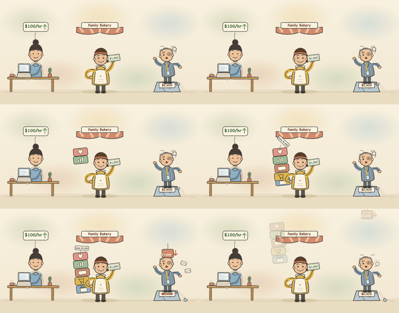
<p><em>Part 5 of <a href="/series/software-scarcity/">The End of Software Scarcity</a>.</em></p>

<p>One of the first things you learn when working with AI is simple: ask for evidence.</p>

<p>I’ve spent the last few months arguing that AI is making software cheaper.</p>

<p>Then I realized I should take my own advice.</p>

<p>Where is the evidence?</p>

<h2 id="simple-economics">Simple Economics</h2>

<p>Here’s the mechanism: when supply rises faster than demand, price falls.</p>

<p>Code supply has visibly risen since coding agents arrived. GitHub’s own <a href="https://github.blog/news-insights/octoverse/octoverse-a-new-developer-joins-github-every-second-as-ai-leads-typescript-to-1/">Octoverse 2025 report</a> puts a number on it: developers pushed nearly <strong>1 billion commits in 2025, up 25.1% year-over-year</strong> — the platform’s biggest jump on record, including almost 100 million commits in August alone. Commits aren’t code exactly, but they’re the closest supply meter we have, and it’s spinning faster than ever.</p>

<p>So: <strong>does that mean software cost is about to come down?</strong></p>

<p>Not evenly. Price isn’t set by supply alone — it’s set by what buyers can substitute for what they already pay. Routine, well-specified work is already getting repriced: demand for AI-substitutable freelance skills is down 20–50% relative to trend, exactly where a price collapse hits first (see References). Bespoke work that used to sit outside the budget becomes affordable — that’s the build-vs-buy shift below. And demand for software was never fixed: cheaper production unlocks buyers who never bought custom software at the old price, eating part of the supply increase. The invoice doesn’t fall uniformly. Software purchasing power beats a price index because it survives demand that moves too.</p>

<h2 id="the-short-version">The Short Version</h2>

<p>There is no single number for “how much cheaper software has become.” The honest evidence is messier and more interesting than that. Developer productivity, labor cost, production cost, market price, and what I’ll call software purchasing power can all move in different directions at once. Below, two strong supporting signals, one important counterexample, and the concept I think actually matters.</p>

<h2 id="what-the-evidence-actually-shows">What the Evidence Actually Shows</h2>

<h3 id="developers-really-can-get-more-done">Developers really can get more done</h3>

<p>The strongest evidence I found is a <a href="https://www.microsoft.com/en-us/research/publication/the-effects-of-generative-ai-on-high-skilled-work-evidence-from-three-field-experiments-with-software-developers/">Microsoft Research field experiment</a> covering 4,867 professional developers. Randomized access to an AI coding assistant increased completed tasks by roughly 26%.</p>

<p>That’s real. But it measures <em>productivity</em> — output per developer — not what anyone paid for the finished software. A 26% productivity gain does not automatically mean a 26% cheaper product.</p>

<h3 id="businesses-are-starting-to-build-instead-of-buy">Businesses are starting to build instead of buy</h3>

<p>The second signal is a build-vs-buy shift. In <a href="https://www.mckinsey.com/capabilities/quantumblack/our-insights/the-state-of-ai">McKinsey’s State of AI</a> survey, about 32% of respondents said their organization had decided <em>against</em> purchasing a software product or feature because agentic coding tools let them build it internally.</p>

<p>That’s a meaningful early signal, not proof. McKinsey didn’t verify that these companies rebuilt an identical commercial product for less. What they reported is a changed decision: build now looks viable where buy used to win by default. That’s still worth taking seriously, because it’s exactly the mechanism my broader thesis depends on.</p>

<h2 id="the-counterevidence-front-and-center">The Counterevidence, Front and Center</h2>

<p>Here’s where it gets uncomfortable for my own argument.</p>

<p><a href="https://metr.org/blog/2025-07-10-early-2025-ai-experienced-os-dev-study/">METR</a> studied 16 experienced open-source developers completing 246 real tasks in mature codebases they already knew well. Using early-2025 AI tools, they took about <strong>19% longer</strong> — even though they <em>believed</em> AI had made them faster.</p>

<p>This is not a small caveat. It suggests the Microsoft/Accenture gains may not generalize to experienced developers doing complex work in codebases they already understand. Greenfield work, junior developers, and well-bounded tasks may behave completely differently from brownfield maintenance on a system an expert already knows cold.</p>

<p>So: productivity gains from AI are real in some settings and absent, or negative, in others. Anyone telling you it’s universal is skipping the METR result.</p>

<h2 id="software-purchasing-power">Software Purchasing Power</h2>

<p>Here’s the reframe I think is more useful than any single percentage.</p>

<p>Instead of asking “how much cheaper is software?”, ask: <strong>how much more software can I buy for $1,000 today than I could two years ago?</strong></p>

<p>The evidence above doesn’t point to invoices falling by some clean number. It points somewhere else: for the same money, you can plausibly get more functionality. A <a href="https://www.goodfirms.co/resources/custom-software-development-cost-survey">GoodFirms survey</a> of software companies found roughly 61% expect AI to cut development costs 10–25% — but it also surfaces something more interesting: some of that saving doesn’t show up as a lower invoice at all. It shows up as scope that used to be out of budget getting included instead.</p>

<p>Same money. More software. That’s technological deflation of the kind we’ve seen before in other industries, where capability rises faster than the sticker price falls.</p>

<h2 id="back-to-the-thesis">Back to the Thesis</h2>

<p>This connects to the claim I made when I started this series: that software scarcity is ending.</p>

<p>The old model was straightforward. Software was expensive to build, so businesses adapted themselves to it:</p>

<p><strong>Business → adapts to → Software</strong></p>

<p>If the marginal cost of building and modifying software keeps falling, that relationship can start to reverse:</p>

<p><strong>Software → adapts to → Business</strong></p>

<p>The McKinsey build-vs-buy number is an early signal of exactly this — companies choosing custom over generic because custom got cheap enough to be worth it. I’m not declaring SaaS dead. I’m saying the calculation is shifting, and I can point to a specific data point instead of just asserting it.</p>

<h2 id="so-how-much-cheaper-has-software-become">So, How Much Cheaper Has Software Become?</h2>

<p>The honest answer is that we don’t have a single number.</p>

<p>In controlled settings, developer output rose by roughly 26%, and other field research has found gains as high as 55%. Software companies expect AI to cut development costs 10–25%. Some freelance categories are already under pricing and demand pressure. Some companies are now building what they used to buy. And experienced developers on complex, familiar codebases saw <em>no</em> gain — some got slower.</p>

<p>None of those numbers means “software is 26% cheaper” or “55% cheaper.” Forcing them into one figure would be the opposite of asking for evidence.</p>

<p>The more interesting possibility is that we’re measuring the wrong thing. The price of software may not collapse. The amount of software we can afford might explode instead.</p>

<p>Historically, software was expensive and ideas were cheap. If software production keeps becoming abundant, that relationship may flip: software becomes cheap, and good ideas become the expensive part.</p>

<p>That, I think, is what the end of software scarcity actually means.</p>

<h2 id="footnote-five-things-that-move-separately">Footnote: Five Things That Move Separately</h2>

<p>Before any of the evidence above makes sense, keep five things separate: developer productivity (output per developer), labor cost (cost of engineering time), production cost (total cost of creating the software), market price (what customers pay), and software purchasing power (functionality per dollar). They don’t move together — an AI-skilled developer can charge more per hour while finishing in far fewer hours, so labor gets pricier per hour while the software gets cheaper to produce. Illustration, not data: before AI, 40 hours × $60/hour = $2,400; with AI, 10 hours × $100/hour = $1,000. Nobody measured this exact project, but it shows productivity, labor cost, and production cost moving in three directions in one paragraph.</p>

<h2 id="references">References</h2>

<p>Additional evidence reviewed for this article, not covered in the body above:</p>

<ul>
  <li><a href="https://www.bis.org/publ/work1208.htm">BIS / Ant Group CodeFuse field experiment</a> — a field experiment found generative AI increased code output by roughly 55%, concentrated among less-experienced developers.</li>
  <li><a href="https://ramp.com/data/ai-labor-market-impact-freelancers">Ramp Economics Lab</a> — businesses with high AI exposure saw roughly $0.03 of increased AI spending for every $1 of reduced freelance spending. This is spending substitution, not proof that AI output equals freelance output.</li>
  <li><a href="https://www.upwork.com/research/research-future-workforce-index-2026">Upwork Future Workforce Index 2026</a> — AI-using freelancers earn about 34% more per hour, while lower-complexity generative-AI contract work saw starts up ~90% and per-contract earnings down ~13%.</li>
  <li><a href="https://www.goodfirms.co/resources/custom-software-development-cost-survey">GoodFirms Custom Software Development Cost Survey</a> — survey of 100+ development companies on AI’s expected effect on cost and scope.</li>
  <li><a href="https://www.sciencedirect.com/science/article/pii/S0167268124004591">Freelance-market research on generative AI</a> — analysis of 3M+ freelance postings found demand for AI-substitutable skills fell 20–50% relative to trend, while complementary AI-skill demand rose.</li>
</ul>]]></content><author><name>Ferosh Jacob</name><email>feroshjacob@gmail.com</email><uri>https://feroshjacob.github.io</uri></author><category term="software-scarcity" /><category term="software-economics" /><category term="ai-assisted-development" /><category term="developer-productivity" /><category term="build-vs-buy" /><category term="software-pricing" /><summary type="html"><![CDATA[I've spent months arguing AI is making software cheaper. So I went looking for the evidence, applied my own rule, and found something more interesting than a percentage: software purchasing power.]]></summary><media:thumbnail xmlns:media="http://search.yahoo.com/mrss/" url="https://feroshjacob.github.io/images/software-cheaper-by-how-much.png" /><media:content medium="image" url="https://feroshjacob.github.io/images/software-cheaper-by-how-much.png" xmlns:media="http://search.yahoo.com/mrss/" /></entry><entry><title type="html">CPU vs GPU battle, Round 1: leave the laptop, the ceiling comes with you</title><link href="https://feroshjacob.github.io/posts/2026/09/13/cpu-vs-gpu-battle-part-4-leave-the-laptop" rel="alternate" type="text/html" title="CPU vs GPU battle, Round 1: leave the laptop, the ceiling comes with you" /><published>2026-09-13T00:00:00+00:00</published><updated>2026-09-13T00:00:00+00:00</updated><id>https://feroshjacob.github.io/posts/2026/09/13/cpu-vs-gpu-battle-part-4-leave-the-laptop</id><content type="html" xml:base="https://feroshjacob.github.io/posts/2026/09/13/cpu-vs-gpu-battle-part-4-leave-the-laptop"><![CDATA[<p><img src="/images/cpu-vs-gpu-battle-part-4.png" alt="Architecture of the Part 4 datacenter-GPU arm: the same (query + product title) pairs and the same byte-for-byte system prompt from Part 1's Arm B are gzipped into Kubernetes ConfigMaps and shipped to a National Research Platform GPU node, where vLLM serves Qwen2.5-7B-Instruct; the generated JSON goes through the identical ported parser and the identical QWK formula, and the scoreboard underneath plots all five arms on one QWK axis, showing a lexical floor near 0.22 and the learned and prompted arms spread between roughly 0.24 and 0.49, with nothing breaking 0.5, regardless of whether the arm ran on a laptop CPU, a laptop GPU, or a datacenter GPU" /></p>

<p><em>Part 4, and the last part of Round 1. Part 1 prompted a small generalist and watched it
miscalibrate. Part 2 trained a specialist that won in-domain. Part 3 adapted a generalist
with LoRA and found the only arm that did not degrade out of domain. All three ran on one
16 GB laptop. This round we finally leave it - same problem, same labels, a real
datacenter GPU - to answer the question the series has been circling since Part 1.</em></p>

<h2 id="the-short-version">The Short Version</h2>

<p><strong>Nothing in this experiment has broken 0.5 QWK</strong> against independent human labels, and
every learned or prompted arm has landed somewhere between 0.24 and 0.49. That is the
whole shape of Round 1: a lexical floor at 0.222, a prompted 3B at 0.288, a fine-tuned
cross-encoder at 0.360, a LoRA-adapted generative model at 0.353 - and the single best
number anywhere, 0.486, out of domain. Four methods that share nothing all landed under
the same 0.5 ceiling, spread across roughly a quarter of the scale rather than clustered
together.</p>

<p>Which leaves one obvious suspect. Every one of those arms was <strong>laptop-bound by design</strong>.
Maybe the ceiling was never the problem. Maybe it was the machine.</p>

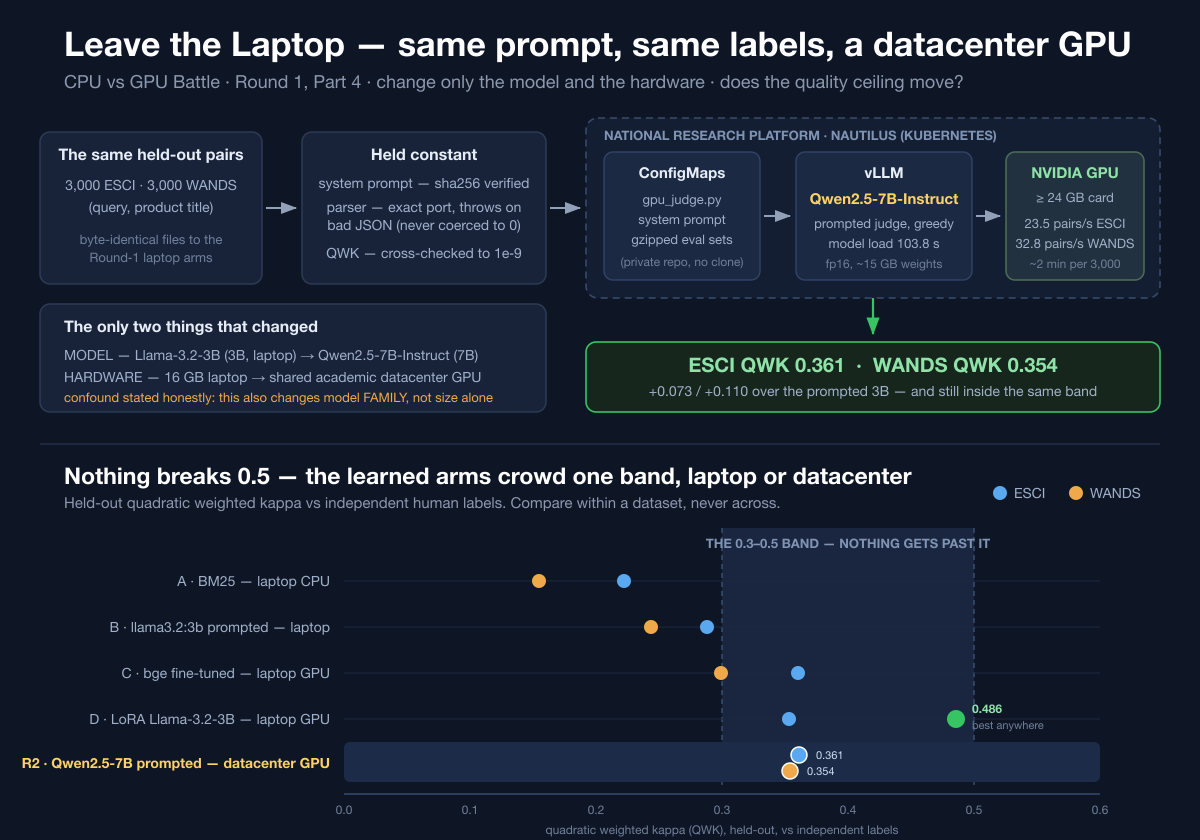
<p>So this round changes exactly two things - the model and the hardware - and nothing else.
A prompted <code class="language-plaintext highlighter-rouge">Qwen2.5-7B-Instruct</code> on a datacenter NVIDIA GPU, served by vLLM, grading the
identical 3,000 held-out ESCI pairs and 3,000 held-out WANDS pairs, with the same system
prompt (verified byte-for-byte by hash), the same parser, and the same QWK implementation
Round 1 used.</p>

<p>The answer:</p>

<ul>
  <li><strong>ESCI QWK 0.361</strong> (95% CI 0.333-0.389), <strong>WANDS QWK 0.354</strong> (95% CI 0.326-0.382).</li>
  <li>Versus the 3B it scaled up from: <strong>+0.073 on ESCI, +0.110 on WANDS</strong>. Real, and not small.</li>
  <li>And landed <strong>inside the 0.24-0.49 band</strong> the learned laptop arms already occupied. It
did not beat Part 3’s 0.486. It did not break anything.</li>
</ul>

<p><strong>The ceiling is the task, not the model size.</strong> Pointwise relevance grading against
independent human labels is genuinely hard, and a 2.3x bigger prompted judge on
datacenter hardware does not change that. That finding is what the whole round was for,
and it is now a poster at the Science and Cyberinfrastructure for Discovery (SCD) 2026 at
Georgia State University - more on that at the end.</p>

<h2 id="where-we-left-off-a-ceiling-nobody-could-break">Where we left off: a ceiling nobody could break</h2>

<p>Round 1’s scorecard after three parts, all of it on one laptop:</p>

<table>
  <thead>
    <tr>
      <th>Arm</th>
      <th>Where it ran</th>
      <th>ESCI QWK</th>
      <th>WANDS QWK</th>
    </tr>
  </thead>
  <tbody>
    <tr>
      <td>A - BM25</td>
      <td>laptop CPU</td>
      <td>0.222</td>
      <td>0.155</td>
    </tr>
    <tr>
      <td>B - prompted <code class="language-plaintext highlighter-rouge">llama3.2:3b</code></td>
      <td>laptop, Ollama</td>
      <td>0.288</td>
      <td>0.244</td>
    </tr>
    <tr>
      <td>C - fine-tuned <code class="language-plaintext highlighter-rouge">bge-reranker-v2-m3</code></td>
      <td>laptop GPU (Metal)</td>
      <td>0.360</td>
      <td>0.299</td>
    </tr>
    <tr>
      <td>D - LoRA <code class="language-plaintext highlighter-rouge">Llama-3.2-3B</code></td>
      <td>laptop GPU (MLX)</td>
      <td>0.353</td>
      <td><strong>0.486</strong></td>
    </tr>
  </tbody>
</table>

<p>Two honest readings were available at the end of Part 3, and they point in opposite
directions:</p>

<ol>
  <li><strong>The task is hard.</strong> Four very different methods - lexical, prompted, discriminative
fine-tune, generative adapter - all landed under the same 0.5 ceiling, with the three
learned or prompted methods filling the 0.24-0.49 range above the lexical floor. When
methods that share nothing land under the same ceiling, the thing they share is the
problem.</li>
  <li><strong>The machines are small.</strong> Every arm fit in 16 GB of unified memory because that was
the constraint we set, not because it was the right size for the job. A 3B model is a
small model. Nobody serious grades relevance with a 3B model if they have a choice.</li>
</ol>

<p>You cannot settle that from inside the laptop. You have to go get a bigger machine.</p>

<h2 id="the-experiment-change-two-things-hold-everything-else">The experiment: change two things, hold everything else</h2>

<p>This is the part that makes the number mean anything. If you change the model <em>and</em> the
prompt <em>and</em> the parser <em>and</em> the scoring, a QWK movement tells you nothing about which
change caused it. So the round was built as an ablation against Part 1’s Arm B, with the
changed surface reduced to <strong>model + hardware</strong>:</p>

<table>
  <thead>
    <tr>
      <th>Held constant</th>
      <th>How it was held</th>
    </tr>
  </thead>
  <tbody>
    <tr>
      <td>Judge <strong>system prompt</strong></td>
      <td>Dumped byte-for-byte out of the production source and shipped as a file. Its <strong>sha256 matched on the laptop and inside the cluster ConfigMap</strong> - not “looks the same,” identical.</td>
    </tr>
    <tr>
      <td>Per-pair <strong>user prompt</strong></td>
      <td>The prompt builder ported function-for-function from JavaScript to Python.</td>
    </tr>
    <tr>
      <td><strong>Parser</strong></td>
      <td>Same port. Strip reasoning tags and code fences, take first <code class="language-plaintext highlighter-rouge">{</code> to last <code class="language-plaintext highlighter-rouge">}</code>, require an integer grade in 0-3, otherwise <strong>throw</strong>. A parse failure is recorded as a failure and <strong>excluded</strong> from QWK - never quietly coerced to 0.</td>
    </tr>
    <tr>
      <td><strong>Eval sets</strong></td>
      <td>The exact same <code class="language-plaintext highlighter-rouge">esci_eval_sample.jsonl</code> and <code class="language-plaintext highlighter-rouge">wands_eval_sample.jsonl</code> files, 3,000 rows each, that every Round-1 arm scored on - gzipped into a ConfigMap and shipped to the cluster.</td>
    </tr>
    <tr>
      <td><strong>QWK</strong></td>
      <td>The scoring function ported and then <strong>cross-checked to 1e-9</strong> against the original JavaScript on seeded arrays before anything was run.</td>
    </tr>
  </tbody>
</table>

<p>The model-delivery mechanism is matched too: Ollama applied <code class="language-plaintext highlighter-rouge">llama3.2</code>’s own instruct
chat template for Arm B, and vLLM’s <code class="language-plaintext highlighter-rouge">chat()</code> applies Qwen’s. Same shape, different model.</p>

<h3 id="the-model-and-an-honest-confound">The model, and an honest confound</h3>

<p>The model I <em>wanted</em> was <strong>Llama-3.1-8B-Instruct</strong> - same family as Arm B’s Llama-3.2-3B,
so 3B to 8B would isolate <strong>size</strong> and only size. It is gated on HuggingFace and no access
token was available in the cluster environment, so it could not be pulled.</p>

<p>The model I <em>used</em> was <strong><code class="language-plaintext highlighter-rouge">Qwen/Qwen2.5-7B-Instruct</code></strong> - open, ungated, and a strong
instruct model at roughly the same scale. That means this run changes model <strong>family</strong> as
well as size. So the +0.073 / +0.110 lift over Arm B is “a bigger, different-family
prompted model,” not a clean size ablation, and I am going to say that every time I quote
the number. The clean version needs one more run with a token in the environment.</p>

<p>It is worth being clear about what the confound does and does not threaten. It muddies the
attribution of the <em>lift</em>. It does not touch the headline, which is a <strong>ceiling</strong> claim: a
strong 7B on datacenter hardware still landed at ~0.35.</p>

<h2 id="getting-onto-a-datacenter-gpu-the-part-nobody-writes-about">Getting onto a datacenter GPU (the part nobody writes about)</h2>

<p>The compute came from the <strong>National Research Platform’s Nautilus cluster</strong> - a shared
academic Kubernetes GPU pool. Writing the judge took an afternoon. Getting a pod onto a
card took three separate fixes, and I think they are more useful to read than the YAML:</p>

<ol>
  <li><strong>Resource ratios.</strong> The cluster enforces that CPU, memory, and ephemeral storage
limits sit within 1.2x of their requests. The fix is to set requests equal to limits
and stop being clever: 3 CPU, 20 GiB memory, 40 GiB ephemeral.</li>
  <li><strong>The big cards are tainted.</strong> 48 GB cards carry a <code class="language-plaintext highlighter-rouge">large-gpu</code> hardware taint, which is
a hardware label, not a preemption one - so tolerating it does not make the job
preemptible. Without the toleration you simply never schedule.</li>
  <li><strong>The pool was too narrow.</strong> The manifest asked for an RTX A6000 by node affinity, and
every A6000 in the cluster was allocated. But Qwen2.5-7B at fp16 is about 15 GB - it
fits any card with 24 GB or more. Widening the affinity to the pool of non-quota-gated
24-48 GB products scheduled it immediately, because the 24 GB tier had dozens of free
cards sitting idle while I queued for the 48 GB one.</li>
</ol>

<p>That third one is the practical lesson of the round: <strong>ask for the GPU your model needs,
not the biggest GPU you can name.</strong> The queue is at the top of the range.</p>

<p>The job itself is deliberately boring and safe for a shared cluster: a <code class="language-plaintext highlighter-rouge">vllm-openai</code>
image with the entrypoint overridden to the judge script, code and data mounted from
ConfigMaps (the repo was private, so no clone), <code class="language-plaintext highlighter-rouge">restartPolicy: Never</code>, <code class="language-plaintext highlighter-rouge">backoffLimit: 0</code>,
and a 2-hour <code class="language-plaintext highlighter-rouge">activeDeadlineSeconds</code> so a hung pod can never idle on a card it is not
using. Results come back on stdout between marker lines and get collected with
<code class="language-plaintext highlighter-rouge">kubectl logs</code>.</p>

<h2 id="the-result-the-ceiling-did-not-move">The result: the ceiling did not move</h2>

<p>Model load took <strong>103.8 seconds</strong>. After that, greedy generation ran at <strong>23.5 pairs/sec</strong>
on ESCI and <strong>32.8 pairs/sec</strong> on WANDS - 3,000 pairs in about two minutes per set.</p>

<p>Here is the full Round-1 scorecard with the datacenter arm in it:</p>

<table>
  <thead>
    <tr>
      <th>Arm</th>
      <th>Hardware</th>
      <th>ESCI QWK</th>
      <th>WANDS QWK</th>
      <th>ESCI acc</th>
      <th>WANDS acc</th>
      <th>Parse fails</th>
    </tr>
  </thead>
  <tbody>
    <tr>
      <td>A - BM25</td>
      <td>laptop CPU</td>
      <td>0.222</td>
      <td>0.155</td>
      <td>0.401</td>
      <td>0.377</td>
      <td>-</td>
    </tr>
    <tr>
      <td>B - prompted <code class="language-plaintext highlighter-rouge">llama3.2:3b</code></td>
      <td>laptop</td>
      <td>0.288</td>
      <td>0.244</td>
      <td>0.317</td>
      <td>0.310</td>
      <td>7 / 11</td>
    </tr>
    <tr>
      <td>C - fine-tuned bge</td>
      <td>laptop GPU</td>
      <td>0.360</td>
      <td>0.299</td>
      <td><strong>0.517</strong></td>
      <td>0.473</td>
      <td>-</td>
    </tr>
    <tr>
      <td>D - LoRA Llama-3.2-3B</td>
      <td>laptop GPU</td>
      <td>0.353</td>
      <td><strong>0.486</strong></td>
      <td>0.483</td>
      <td><strong>0.603</strong></td>
      <td>-</td>
    </tr>
    <tr>
      <td><strong>R2 - prompted Qwen2.5-7B</strong></td>
      <td><strong>datacenter GPU</strong></td>
      <td><strong>0.361</strong></td>
      <td>0.354</td>
      <td>0.343</td>
      <td>0.332</td>
      <td>3 / 0</td>
    </tr>
  </tbody>
</table>

<p>Read down a column, never across - ESCI and WANDS use different label spaces.</p>

<p>The bigger prompted model on the bigger machine scored <strong>0.361 and 0.354</strong>. Arm C, a
fine-tuned cross-encoder that runs in about a gigabyte of RAM on a laptop, scored <strong>0.360</strong>
on ESCI. Those two numbers are the same number. The 95% confidence intervals - [0.333,
0.389] and [0.326, 0.382] - sit right on top of the band the laptop fine-tunes were already in.</p>

<p><strong>So the answer to the question that closed Part 3 is: the ceiling is the task.</strong> Scaling
the prompted judge 2.3x and moving it onto a card with more memory than the entire laptop
moved it from one part of the 0.24-0.49 band to another part of the same band. Pointwise
relevance grading against independent human labels is hard in a way that more parameters
do not fix.</p>

<h2 id="where-the-bigger-model-genuinely-did-help">Where the bigger model genuinely did help</h2>

<p>I do not want the headline to flatten a real result. Against Arm B - identical method,
identical prompt, identical parser, just 3B instead of 7B and a laptop instead of a
cluster - QWK rose <strong>+0.073 on ESCI</strong> (0.288 to 0.361) and <strong>+0.110 on WANDS</strong> (0.244 to
0.354). Scale helps <em>inside</em> the band, and it helps by a lot.</p>

<p>The more interesting consequence is what that buys you with <strong>no training at all</strong>. The
prompted 7B:</p>

<ul>
  <li><strong>Ties the fine-tuned cross-encoder on ESCI</strong> - 0.361 vs 0.360, in-domain, on the data
the cross-encoder was fine-tuned on.</li>
  <li><strong>Beats it out of domain on WANDS</strong> - 0.354 vs 0.299.</li>
</ul>

<p>A model that never saw a single labeled example from this task matched a purpose-built
fine-tune on its home turf and generalized better off it. If you have GPU access and no
labeled data, that is a genuinely useful place to start, and it is the strongest practical
argument in this round for reaching for the bigger machine.</p>

<h2 id="where-it-loses-because-it-does">Where it loses (because it does)</h2>

<ul>
  <li><strong>It did not catch the LoRA out of domain.</strong> WANDS: 0.354 vs Part 3’s <strong>0.486</strong>. This is
the sharpest loss in the round and the clearest evidence the ceiling held - the best
number in the whole experiment still belongs to a 3B model that was adapted on a laptop
before dinner. A bigger prompted judge on better hardware did not get near it.</li>
  <li><strong>It loses badly on exact accuracy to both fine-tunes.</strong> 0.343 / 0.332, against bge’s
0.517 / 0.473 and the LoRA’s 0.483 / 0.603. Its QWK is respectable only because its
mistakes are ordinally <em>close</em>: off-by-one accuracy 0.79 on ESCI and 0.87 on WANDS, MAE
0.91 and 0.80. It agrees with the humans about <strong>rank</strong> far better than about <strong>label</strong>.</li>
  <li><strong>You can see why in the prediction distribution: it hugs the middle.</strong> On WANDS it
predicted grade 3 only <strong>148 times out of 3,000</strong>, and grade 1 <strong>1,469 times</strong>. On ESCI
it used grade 3 only 479 times out of 2,997. A judge that will not commit to “exactly
relevant” gets the ordering roughly right and the label consistently wrong.</li>
  <li><strong>Deployment cost is in a different universe.</strong> This needs a 24 GB-or-larger datacenter
GPU and a 104-second model load. Throughput is excellent once it is warm - 23 to 33
pairs/sec batched - but Arm C does about <strong>28 ms/pair in ~1 GB</strong> on a laptop. For a
shipping on-device judge, the cross-encoder still wins the efficiency trade by a wide
margin, and it is not close.</li>
  <li><strong>It wrote three pieces of invalid JSON.</strong> Three parse failures on ESCI, zero on WANDS,
all the same failure mode: the model put a literal unescaped <code class="language-plaintext highlighter-rouge">"</code> inside its <code class="language-plaintext highlighter-rouge">reason</code>
string - an inch mark in <code class="language-plaintext highlighter-rouge">40"</code>, or quoting the query <code class="language-plaintext highlighter-rouge">"cream and sugar"</code> back at itself.
A prompted judge that writes free-text reasons will occasionally produce unparseable
output. The parser rejected all three rather than inventing a grade, which is the
correct behavior and is exactly why they are reported here instead of silently becoming
zeros.</li>
</ul>

<h2 id="why-i-did-not-run-a-14b">Why I did not run a 14B</h2>

<p>The plan going in was explicit: run ~8B first, go to 14B <strong>only if the ceiling visibly
moved</strong>, and do not jump to 70B or A100-class hardware unless the trend was clear.</p>

<p>It did not move. The 7B landed on the same ~0.35 plateau as two 3B fine-tunes, and the 3B
to 7B trend is already showing diminishing returns inside the band. A 14B prompted judge
would very likely land in the same band at more cost, on a shared academic cluster where
that GPU-hour is somebody else’s queue. So I did not spend it. The manifest is one
<code class="language-plaintext highlighter-rouge">--model</code> change away if the datapoint is ever worth having.</p>

<p>Reporting a negative result and then <em>not</em> buying a bigger one to dress it up is, I think,
the whole point of keeping an honest scorecard.</p>

<h2 id="honest-caveats-they-travel-with-every-round">Honest caveats (they travel with every round)</h2>

<ul>
  <li><strong>Compare arms within a dataset, never across.</strong> ESCI and WANDS use different label
spaces - WANDS has no grade 1 at all - and are not on the same scale. Read down a column.</li>
  <li><strong>Family confound, restated.</strong> Qwen2.5-7B vs Llama-3.2-3B mixes family with size. The
lift is “bigger and different,” not “bigger.” The ceiling claim is unaffected.</li>
  <li><strong>This is still an on-device contest at heart.</strong> The shipped production default is
cloud-first (a hosted Gemini model), which was <strong>not</strong> benchmarked in this experiment and
would very likely beat every arm here, including this one. What Round 1 asked was
narrower: what is the best relevance judge you can get without an API call, and does
leaving the laptop change the answer.</li>
  <li><strong>Agreement with the production system’s own history is reproduction, not accuracy</strong> -
the circularity trap from Part 1 holds for every round, which is why every number in this
series is scored against independent labels.</li>
  <li><strong>One run per arm, 3,000 pairs per set.</strong> The confidence intervals are bootstrap
intervals over that sample, not variance across repeated runs. Greedy decoding makes the
run reproducible; it does not make the sample bigger.</li>
</ul>

<h2 id="where-this-went-a-poster-at-scd-2026">Where this went: a poster at SCD 2026</h2>

<p>This finding - that the quality ceiling is a property of the task rather than of model
size - was written up with <strong>Jiho Noh</strong> (Department of Computer Science, Kennesaw State
University) as <em>“The Quality Ceiling Is the Task, Not the Model Size: A Reproducible
CPU/GPU Benchmark of Search-Relevance Judges,”</em> and it was <strong>accepted as a poster at SCD
2026 at Georgia State University</strong>, with a 3-minute lightning talk in the Artificial
Intelligence and Machine Learning session on September 22.</p>

<p>The poster is the compressed version of all four parts: one pipeline, one label mapping
taken from the production system’s own source rather than retyped, one metric, and every
arm scored identically across three hardware tiers. If you want the argument on a single
page instead of across four posts, that is the page.</p>

<h2 id="next-round-1-closes-the-battle-does-not">Next: Round 1 closes, the battle does not</h2>

<p>Four parts in, Round 1 has an answer, and it is a negative one - which is usually the kind
worth having. The ceiling on pointwise relevance grading is the task. It survived a
lexical baseline, a prompted small model, a discriminative fine-tune, a generative
adapter, and a 2.3x bigger prompted judge on a datacenter GPU. Five methods, three
hardware tiers, one ceiling nobody broke.</p>

<p>What that leaves you with is not “which model is best” but <strong>which arm is best for which
goal</strong>, and the series has a clear answer to that now:</p>

<ul>
  <li><strong>Shipping an on-device judge for one domain?</strong> The Part 2 cross-encoder. 28 ms, 1 GB,
best in-domain accuracy of anything here.</li>
  <li><strong>Grading queries from domains you did not train on?</strong> The Part 3 LoRA. Still holds the
best number in the experiment, and it holds it on a laptop.</li>
  <li><strong>No labeled data, but you have GPU access?</strong> This round’s prompted 7B. It ties a
fine-tune in-domain with zero training.</li>
  <li><strong>Need to actually break 0.5?</strong> Nothing here does it. That needs a different problem
formulation - pairwise or listwise comparison instead of pointwise grading, or richer
inputs than a query and a product title - not a bigger model.</li>
</ul>

<p>Two things Round 1 earned but did not run, and I would rather list them than pretend they
are done: the clean same-family size ablation (Llama-3.1-8B, once there is a token in the
cluster environment), and the reverse generalization test Part 3 asked for - train on
WANDS, test on ESCI - which is the real proof that adapting a generalist travels.</p>

<p>The battle itself is open-ended. Round 1 took search relevance. Round 2 takes a different
problem, and the CPU gets to swing first again.</p>

<p><em>Same rules every round: independent labels, held-out numbers, and the losses reported
next to the wins.</em></p>

<p>Code and reproduction details: <a href="https://github.com/Northvalley-Intelligence/cortex/tree/main/experiments/relevancy-replacement">github.com/Northvalley-Intelligence/cortex</a> — journals 00-08 and <code class="language-plaintext highlighter-rouge">results/*.json</code> on <code class="language-plaintext highlighter-rouge">main</code>; this round’s <a href="https://github.com/Northvalley-Intelligence/cortex/blob/round2-gpu-arm/experiments/relevancy-replacement/09-round2-gpu-arm.md">journal 09</a>, the Kubernetes manifest, and the raw <code class="language-plaintext highlighter-rouge">gpu_prompt_qwen2.5-7b__round2.json</code> on the <code class="language-plaintext highlighter-rouge">round2-gpu-arm</code> branch.</p>]]></content><author><name>Ferosh Jacob</name><email>feroshjacob@gmail.com</email><uri>https://feroshjacob.github.io</uri></author><category term="cpu-vs-gpu-battle" /><category term="search-relevance" /><category term="llm-as-judge" /><category term="datacenter-gpu" /><category term="vllm" /><category term="kubernetes" /><category term="benchmarking" /><summary type="html"><![CDATA[Three rounds of this experiment lived on a 16 GB laptop and nothing broke 0.5 QWK - a lexical floor at 0.222, and every learned or prompted arm crowded between 0.24 and 0.49. So we left the machine: the same prompt, the same parser, the same 3,000 held-out pairs, handed to a 7B judge on a datacenter GPU. It scored ESCI QWK 0.361 and WANDS 0.354 - better than the 3B it scaled up from, and still inside the same band. The ceiling is the task, not the model size. The result is now a poster at SCD 2026.]]></summary><media:thumbnail xmlns:media="http://search.yahoo.com/mrss/" url="https://feroshjacob.github.io/images/cpu-vs-gpu-battle-part-4.png" /><media:content medium="image" url="https://feroshjacob.github.io/images/cpu-vs-gpu-battle-part-4.png" xmlns:media="http://search.yahoo.com/mrss/" /></entry><entry><title type="html">CPU vs GPU battle, Round 1: adapt the generalist, read the logits</title><link href="https://feroshjacob.github.io/posts/2026/09/06/cpu-vs-gpu-battle-part-3-adapt-the-generalist" rel="alternate" type="text/html" title="CPU vs GPU battle, Round 1: adapt the generalist, read the logits" /><published>2026-09-06T00:00:00+00:00</published><updated>2026-09-06T00:00:00+00:00</updated><id>https://feroshjacob.github.io/posts/2026/09/06/cpu-vs-gpu-battle-part-3-adapt-the-generalist</id><content type="html" xml:base="https://feroshjacob.github.io/posts/2026/09/06/cpu-vs-gpu-battle-part-3-adapt-the-generalist"><![CDATA[<p><img src="/images/cpu-vs-gpu-battle-part-3.png" alt="Architecture of the Part 3 LoRA relevance judge (Arm D): a (query + product title) pair becomes a chat-template prompt that ends with no trailing space, then feeds a Llama-3.2-3B-Instruct 4-bit base model shown frozen (locked) - the only trainable part is a small pair of low-rank LoRA adapter matrices A and B (rank r) injected into each of the 16 transformer layers, so the layer computes h = W&#183;x + B&#183;A&#183;x with W frozen. At the output, the model's logits at the last token position are read over just the four label tokens (ids 15/16/17/18 = &quot;0&quot;/&quot;1&quot;/&quot;2&quot;/&quot;3&quot;) and an argmax gives the 0-3 grade. A zoom-in shows the frozen full-size weight matrix beside the thin trainable LoRA detour, with the base frozen at ~1.9 GB and training peaking ~5.5 GB on a 16 GB laptop" /></p>

<p><em>Part 3 of the series. Part 1 prompted a generalist and watched it miscalibrate.
Part 2 trained a specialist and watched it win in-domain but travel less well.
This round we try the third thing: keep the generalist, but stop prompting it -
LoRA-tune it on the laptop GPU and read the grade straight off the logits.</em></p>

<h2 id="the-short-version">The Short Version</h2>

<p>Part 2’s cross-encoder was the first arm to beat the shipped on-device judge, but
it was a <strong>specialist</strong> - trained on Amazon ESCI product search, and you could see
it leaning on that domain when it met furniture (WANDS). This round asks the
opposite question: instead of building a purpose-made classifier, can we take the
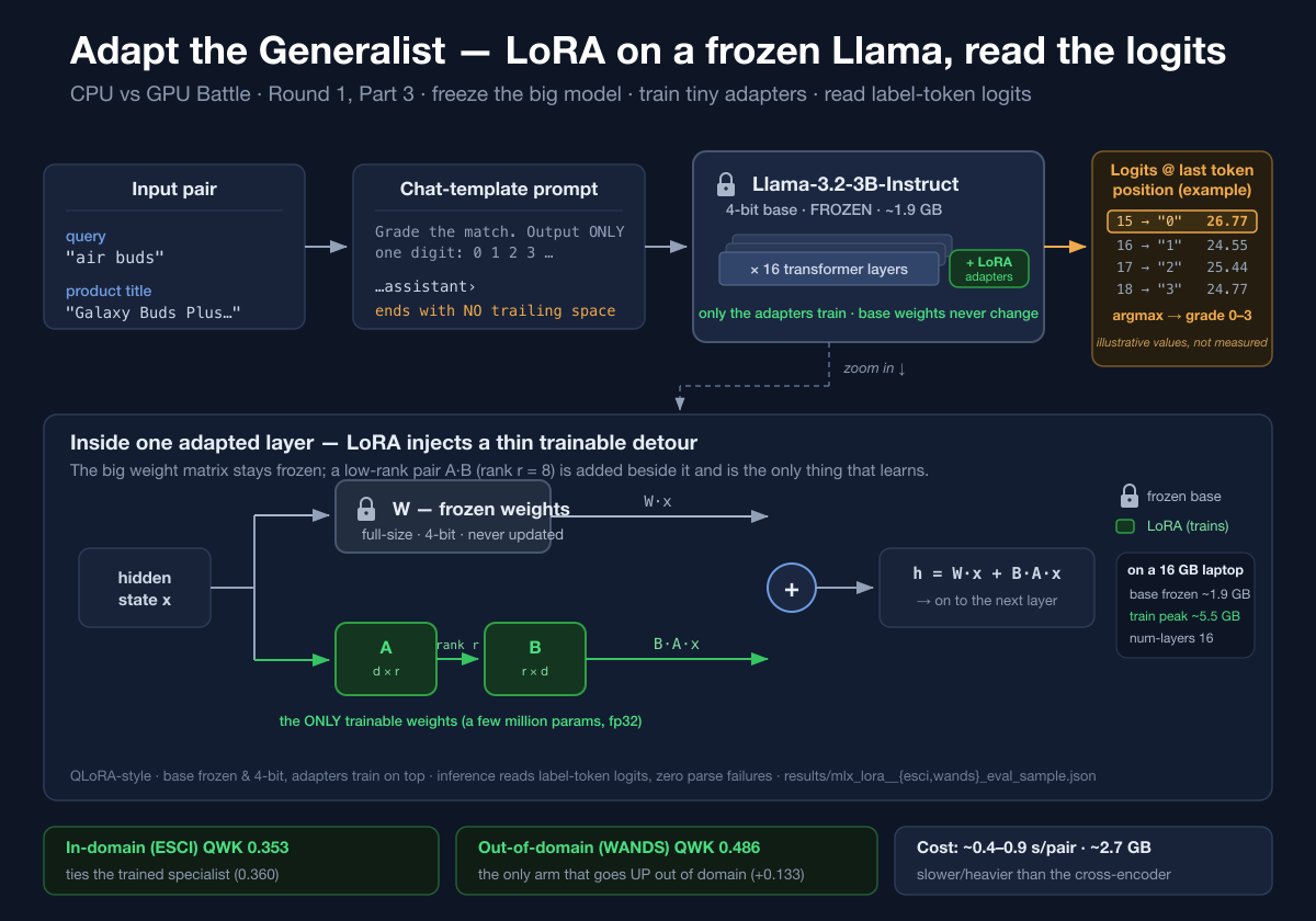
<em>generative</em> model from Part 1 - <code class="language-plaintext highlighter-rouge">Llama-3.2-3B</code> - and <strong>adapt</strong> it into a grader
with a small LoRA, still entirely on the laptop’s GPU?</p>

<p>Two changes make that work on a 16 GB machine:</p>

<ul>
  <li><strong>LoRA on a 4-bit base.</strong> We freeze a 4-bit quantized Llama-3.2-3B (~1.9 GB on
disk) and train only small low-rank adapters on top - QLoRA-style, via
Apple’s <a href="https://github.com/ml-explore/mlx-lm"><code class="language-plaintext highlighter-rouge">mlx_lm</code></a>. Training peaked at
about <strong>5.5 GB of RAM</strong>, comfortable on a 16 GB laptop.</li>
  <li><strong>Read the logits, don’t generate text.</strong> At inference we don’t ask the model to
write JSON. The digits <code class="language-plaintext highlighter-rouge">0 1 2 3</code> are single tokens; we read the model’s logits
for those four tokens at the one position where the grade goes and take the
argmax. No free generation, no parsing, <strong>zero parse failures</strong>.</li>
</ul>

<p>The result is the interesting one of the series so far. In-domain, the adapted
generalist lands about <strong>even</strong> with the trained specialist (ESCI QWK <strong>0.353</strong> vs
the cross-encoder’s 0.360). But out of domain it is the <strong>only arm that does not
fall</strong>: on WANDS it scores QWK <strong>0.486</strong>, while BM25, the prompted model, and the
cross-encoder all drop from their ESCI numbers. That is a lead worth chasing, not a
victory lap - and below I am careful about why.</p>

<p><em>(Numbers: <code class="language-plaintext highlighter-rouge">results/mlx_lora__{esci,wands}_eval_sample.json</code>; journal
<code class="language-plaintext highlighter-rouge">07-arm-d-lora.md</code>. n = 3,000 pairs per set, held-out, independent human labels.)</em></p>

<h2 id="where-we-left-off-a-specialist-that-showed-its-seams">Where we left off: a specialist that showed its seams</h2>

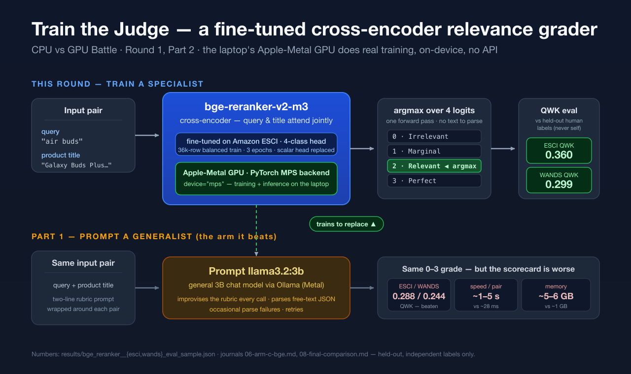
<p>Part 2’s <code class="language-plaintext highlighter-rouge">bge-reranker-v2-m3</code> cross-encoder won the deployment tradeoff outright -
more accurate than the prompted judge <em>and</em> ~200x faster - but it ended on a crack.
Its edge on WANDS furniture (QWK 0.299) was real but thinner than on its home turf,
ESCI (0.360). That is the classic shape of a model that fit its training domain
well and travels less well. A cross-encoder with a bolted-on 4-class head has no
choice: it only knows what it was trained on.</p>

<p>So the Part 3 move is to keep the broad prior knowledge a general chat model already
has - it has “seen” furniture, electronics, and negation queries in pre-training -
and just teach it <em>this scale</em> with a light touch, rather than building a classifier
from the domain up.</p>

<h2 id="the-idea-adapt-a-generalist-instead-of-training-a-specialist">The idea: adapt a generalist instead of training a specialist</h2>

<blockquote>
  <p><strong>New to LoRA?</strong> LoRA (Low-Rank Adaptation) is a way to teach a model a new skill
without retraining all of its billions of weights. You <strong>freeze</strong> the original
model untouched and slip small pairs of low-rank matrices - the <em>adapters</em> - into
its layers; only those tiny matrices ever get trained. Here it’s the QLoRA flavor:
the base Llama is 4-bit quantized and frozen (~1.9 GB), and the adapters train on
top (peaking ~5.5 GB on a 16 GB Apple-Silicon laptop, 16 layers adapted). The
payoff is that the trainable part is tiny and quick to train, and because the base
model stays intact you can keep it and swap a different adapter in for a different
task.</p>
</blockquote>

<p>There are three genuinely different ways to turn a <code class="language-plaintext highlighter-rouge">(query, product title)</code> pair
into a grade, and this series has now built all three. Side by side:</p>

<table>
  <thead>
    <tr>
      <th>Approach</th>
      <th>How it judges</th>
      <th>Training</th>
      <th>This-round result</th>
    </tr>
  </thead>
  <tbody>
    <tr>
      <td><strong>1 · Prompted generalist</strong> — <code class="language-plaintext highlighter-rouge">llama3.2:3b</code> (Part 1)</td>
      <td>Zero-shot: <em>generates</em> JSON, you parse the digit back out</td>
      <td>None — off the shelf</td>
      <td>ESCI QWK 0.288 · WANDS 0.244</td>
    </tr>
    <tr>
      <td><strong>2 · Trained specialist</strong> — <code class="language-plaintext highlighter-rouge">bge</code> cross-encoder (Part 2)</td>
      <td>Argmax over a bolted-on 4-class head — discriminative, no text</td>
      <td>Whole model fine-tuned on ESCI, Apple-Metal (MPS) GPU</td>
      <td>ESCI QWK <strong>0.360</strong> · WANDS 0.299</td>
    </tr>
    <tr>
      <td><strong>3 · Adapted generalist</strong> — <code class="language-plaintext highlighter-rouge">Llama-3.2-3B</code> + LoRA (this round)</td>
      <td>Reads the four label-token logits, argmax — no generation</td>
      <td>LoRA adapters only, frozen 4-bit base, on the GPU</td>
      <td>ESCI QWK 0.353 · WANDS <strong>0.486</strong></td>
    </tr>
  </tbody>
</table>

<p>The same contrast in words:</p>

<ul>
  <li><strong>Approach 1 - prompt a generalist (Part 1).</strong> Take <code class="language-plaintext highlighter-rouge">llama3.2:3b</code> off the shelf,
hand it a two-line rubric, and ask it to <em>generate</em> a grade as JSON. No training.
It improvises the rubric on every call, and you have to parse free text back out.</li>
  <li><strong>Approach 2 - train a specialist (Part 2).</strong> Take a cross-encoder, replace its
head with four class logits, and fine-tune the whole thing on ESCI. It is
<em>discriminative</em> - it does not generate anything, it scores. One forward pass, an
argmax, no text.</li>
  <li><strong>Approach 3 - adapt a generalist (this round).</strong> Take the generative
<code class="language-plaintext highlighter-rouge">Llama-3.2-3B</code>, add LoRA adapters, and train <em>only</em> those on ESCI so the frozen
base keeps its general knowledge. Then, at inference, skip generation entirely and
read the label-token logits. A generative model turned into a judge by
<strong>adaptation</strong>, not by prompting and not by rebuilding.</li>
</ul>

<p>The point of Approach 3 is to get the reliability of a classifier (no parsing, no
malformed output) <em>without</em> throwing away the broad prior that a general model
carries into domains the training set never covered.</p>

<h2 id="how-you-read-a-grade-off-the-logits">How you read a grade off the logits</h2>

<p>This is the mechanic that makes the arm honest, so it is worth being concrete. In
this tokenizer, <code class="language-plaintext highlighter-rouge">"0"</code>, <code class="language-plaintext highlighter-rouge">"1"</code>, <code class="language-plaintext highlighter-rouge">"2"</code>, <code class="language-plaintext highlighter-rouge">"3"</code> each encode to a <strong>single</strong> token (ids
15, 16, 17, 18 - a leading space would split them into two tokens, so the prompt is
built to avoid one). The chat template ends the prompt right where the assistant’s
answer begins, with no trailing space, so the <em>very next token position</em> is
unambiguously the grade digit.</p>

<p>That means we never let the model talk. We run one forward pass over the prompt,
look at the logits for exactly those four token ids at that final position, and take
the argmax. For a given pair the model emits four label-token logits and we take
the largest - they might look like <code class="language-plaintext highlighter-rouge">[26.77, 24.55, 25.44, 24.77]</code> (illustrative,
not measured values), where the argmax lands on grade 0.</p>

<p>Two consequences fall out for free:</p>

<ul>
  <li><strong>No parse failures, ever.</strong> The results file records <code class="language-plaintext highlighter-rouge">parse_failure_count: 0</code>
with the note <em>“not applicable - argmax over the 4 label-digit token logits at one
forward-pass position, no free-generation or text parsing.”</em> Part 1’s prompted arm
had to strip <code class="language-plaintext highlighter-rouge">&lt;think&gt;</code> tags and fences and occasionally threw a pair away; a
logit read cannot malform its output, exactly like Part 2’s classifier.</li>
  <li><strong>It is a fair comparison of <em>method</em>, not data.</strong> Arm D trains on the <em>identical</em>
36k-row balanced ESCI split the Part 2 cross-encoder used (a 4k dev split held
aside), so Approach 2 vs Approach 3 is a clean comparison of <em>cross-encoder
classifier</em> against <em>generative LoRA logit-read</em>, not of who got the better
training rows.</li>
</ul>

<h2 id="training-it-on-the-laptop-gpu">Training it on the laptop GPU</h2>

<p>The GPU does real work again this round. On the Apple-Metal GPU via <code class="language-plaintext highlighter-rouge">mlx_lm</code>, we
LoRA-tune the 4-bit base for one full epoch (9,000 iterations over the 36k rows,
batch size 4, <code class="language-plaintext highlighter-rouge">--num-layers 16</code>, learning rate 1e-5), computing the loss <strong>only on
the completion digit</strong> (<code class="language-plaintext highlighter-rouge">--mask-prompt</code>), not on the instruction text. On a 16 GB
machine the run peaked at about <strong>5.5 GB of RAM</strong> and took a handful of hours - the
kind of job you start before dinner and read the next morning, no datacenter, no API.</p>

<p>The 4-bit base is a deliberate choice, not a shortcut: an fp16 3B model is ~6-7 GB
in weights alone, which leaves almost no headroom for activations and optimizer
state on a 16 GB laptop. Freezing a 4-bit base and training fp32 LoRA adapters on
top is <code class="language-plaintext highlighter-rouge">mlx_lm</code>’s well-supported path and the reason this fits at all.</p>

<p>As always in this series, every score below is measured against <strong>independent
human-derived labels</strong> (Amazon ESCI and WANDS), never the service’s own past
judgments - roughly 92% of those were written by the same local model, so agreeing
with them would measure reproduction, not accuracy. That circularity trap from
Part 1 still governs every number here.</p>

<h2 id="does-it-win-in-domain-it-ties-out-of-domain-it-holds">Does it win? In-domain it ties; out of domain it holds</h2>

<p>Here is the whole board, all four arms this series has built, on the same seeded
held-out samples. Compare arms <em>down a column</em> (within one dataset) - the ESCI and
WANDS columns are <strong>not</strong> on the same ruler, and I say why right after the table.</p>

<table>
  <thead>
    <tr>
      <th>Arm</th>
      <th>ESCI QWK</th>
      <th>WANDS QWK</th>
      <th>ESCI → WANDS</th>
      <th>speed / pair</th>
      <th>memory</th>
    </tr>
  </thead>
  <tbody>
    <tr>
      <td>A · BM25 lexical</td>
      <td>0.222</td>
      <td>0.155</td>
      <td>–0.067</td>
      <td>instant</td>
      <td>tiny</td>
    </tr>
    <tr>
      <td>B · Prompted <code class="language-plaintext highlighter-rouge">llama3.2:3b</code> (≈ shipped judge)</td>
      <td>0.288</td>
      <td>0.244</td>
      <td>–0.044</td>
      <td>~1–5 s</td>
      <td>~5–6 GB</td>
    </tr>
    <tr>
      <td>C · bge cross-encoder, fine-tuned (Part 2)</td>
      <td><strong>0.360</strong></td>
      <td>0.299</td>
      <td>–0.061</td>
      <td><strong>~28 ms</strong></td>
      <td><strong>~1 GB</strong></td>
    </tr>
    <tr>
      <td><strong>D · Llama-3.2-3B + LoRA, logit-read (this round)</strong></td>
      <td>0.353</td>
      <td><strong>0.486</strong></td>
      <td><strong>+0.133</strong></td>
      <td>~0.4–0.9 s</td>
      <td>~2.7 GB</td>
    </tr>
  </tbody>
</table>

<p><em>(Arm D: ESCI QWK 0.353, 95% CI 0.320-0.385, accuracy 0.483, off-by-one 0.722,
mean nDCG 0.840; WANDS QWK 0.486, 95% CI 0.453-0.517, accuracy 0.603, off-by-one
0.816, mean nDCG 0.884 - all from <code class="language-plaintext highlighter-rouge">results/mlx_lora__{esci,wands}_eval_sample.json</code>,
inference peak RSS ~2.67 GB, warm median ~0.87 s/pair on ESCI. Arms A-C from
Parts 1-2 and <code class="language-plaintext highlighter-rouge">results/bge_reranker__*.json</code>.)</em></p>

<p>Read the last two columns together, because that is where the story lives:</p>

<ul>
  <li><strong>In-domain, the adapted generalist ties the specialist.</strong> On ESCI, Arm D’s 0.353
and Arm C’s 0.360 sit inside each other’s confidence intervals (D: 0.320-0.385).
Building the grader by <em>adapting a generalist</em> got essentially the same in-domain
accuracy as <em>training a purpose-built classifier</em>. That alone is a result: you did
not have to give up the general model to get classifier-grade reliability.</li>
  <li><strong>Out of domain, it is the only arm that goes up.</strong> Every other arm loses ground
from ESCI to WANDS - BM25 -0.067, the prompted model -0.044, the specialist
cross-encoder -0.061. Arm D moves the <em>other</em> way: <strong>+0.133</strong>. It is the single
arm in the whole experiment whose ordinal agreement improves on a domain it never
trained on.</li>
</ul>

<h2 id="why-0486--0353-is-a-lead-not-a-trophy">Why “0.486 &gt; 0.353” is a lead, not a trophy</h2>

<p>I want to be exact about what that +0.133 does and does not prove, because it is the
easiest number in this series to over-claim.</p>

<ul>
  <li><strong>You cannot compare the two datasets directly.</strong> WANDS uses a coarser 3-class
label space (Exact / Partial / Irrelevant, no grade-1 bin), which is simply an
easier target than ESCI’s four grades. So “0.486 on WANDS beats 0.353 on ESCI” is
<strong>not</strong> a valid sentence - they are different rulers. The claim is <em>not</em> that Arm D
is better on WANDS than on ESCI in absolute terms.</li>
  <li><strong>What <em>is</em> comparable is the direction, across arms.</strong> Every arm was scored on the
same two rulers. Three of the four degrade going out of domain; one does not. That
cross-arm <em>pattern</em> - who holds up and who slides - is a fair comparison even when
the absolute cross-dataset numbers are not. Arm D holding up (indeed improving) is
the honest signal.</li>
  <li><strong>One out-of-domain collection is not proof of generalization.</strong> WANDS is a single
domain (furniture). A model that travels well to one new domain has earned a
hypothesis, not a law. The real test is a <strong>reverse run</strong> - train on WANDS, test on
ESCI - and see whether the adapted generalist still holds up when the home and away
fields are swapped. That is deliberately left as future work; I would rather flag
it than quietly bank the win.</li>
</ul>

<p>So the fair summary is: <em>adapting a generalist looks like it may travel better than
training a specialist</em> - a lead strong enough to chase, on the strength of being the
only arm that did not degrade out of domain, and honest enough to admit it rests on
one collection and a coarser label space.</p>

<h2 id="where-it-loses-because-it-does">Where it loses (because it does)</h2>

<ul>
  <li><strong>It did not beat the specialist in-domain.</strong> On ESCI, Arm C is still nominally
ahead (0.360 vs 0.353), even if the gap is inside the noise. If ESCI product
search were the only domain you cared about, Part 2’s cross-encoder is still the
arm to ship - and it is far cheaper to run.</li>
  <li><strong>It is slower and heavier than the specialist.</strong> A generative 3B forward pass -
even reading a single position - runs at roughly <strong>0.4-0.9 s/pair</strong> and ~2.7 GB of
RAM at inference, versus the cross-encoder’s ~28 ms and ~1 GB. That is much faster
than Part 1’s prompted arm (seconds, and it actually generated text), but it is
still one to two orders of magnitude off the specialist. Adaptation buys
generalization; it does not buy the classifier’s speed.</li>
  <li><strong>The absolute ceiling is still modest.</strong> QWK in the low-to-mid 0.3s (ESCI) is
<em>better</em>, not <em>good</em>. Every arm in this experiment lives in the ~0.3-0.5
neighborhood; a lead over the baseline is not a solved problem, and I am not going
to dress it up as one.</li>
</ul>

<h2 id="honest-caveats-they-travel-with-every-round">Honest caveats (they travel with every round)</h2>

<ul>
  <li><strong>Compare arms within a dataset, never across.</strong> Restating it because it is the
one that makes the headline honest: the ESCI and WANDS columns use different label
spaces and are not on the same scale. Read down a column.</li>
  <li><strong>This is an on-device contest, not “we beat the cloud.”</strong> The shipped service
default is cloud-first (a hosted Gemini model), which was <strong>not</strong> benchmarked here
and would very likely beat every laptop-bound arm. The win we chase is narrow and
specific: the best relevance grader that runs on <em>this machine</em> with no API call -
for privacy, cost, and offline reasons.</li>
  <li><strong>The GPU is the Apple M-series integrated GPU (Metal), not a discrete card.</strong> No
hand-written CUDA or Metal kernels - <code class="language-plaintext highlighter-rouge">mlx_lm</code> handles device dispatch. The whole
thing, training and inference, fits on a 16 GB laptop, which is the entire point.</li>
  <li><strong>Agreement with the service’s own history is reproduction, not accuracy</strong> - the
circularity trap from Part 1 still holds, which is why every number here is against
independent labels.</li>
</ul>

<h2 id="next-leave-the-laptop">Next: leave the laptop</h2>

<p>Three rounds in, the on-device picture is clear enough to name a winner <em>per goal</em>:
if you only serve ESCI-shaped product search, the Part 2 cross-encoder is the arm -
fastest, lightest, best in-domain. But if you care about grading queries from
domains you did not train on, the adapted generalist is the one that did not fall
over, and that is the more interesting lead.</p>

<p>The open question the whole series has been circling is still open: is the
~0.3-0.5 QWK ceiling the <strong>task</strong> - pointwise relevance grading is just hard - or is
it the <strong>size</strong> of a model that fits on a laptop? Every arm so far has been
laptop-bound by design. In <strong>Part 4</strong> we finally leave the machine and hand the same
problem, the same held-out labels, to a real datacenter GPU - to find out whether
the ceiling moves when the hardware does. And somewhere in there is the reverse
generalization test this round earned but did not run.</p>

<p><em>Same rules every round: independent labels, held-out numbers, and the losses
reported next to the wins.</em></p>

<p>Code and reproduction details: <a href="https://github.com/Northvalley-Intelligence/cortex/tree/main/experiments/relevancy-replacement">github.com/Northvalley-Intelligence/cortex/tree/main/experiments/relevancy-replacement</a> — journals 00-08 and <code class="language-plaintext highlighter-rouge">results/*.json</code>.</p>]]></content><author><name>Ferosh Jacob</name><email>feroshjacob@gmail.com</email><uri>https://feroshjacob.github.io</uri></author><category term="cpu-vs-gpu-battle" /><category term="search-relevance" /><category term="llm-as-judge" /><category term="lora" /><category term="mlx" /><category term="gpu" /><category term="fine-tuning" /><summary type="html"><![CDATA[Part 2 trained a specialist cross-encoder that won in-domain but leaned on its training data. This round we take the generative Llama-3.2-3B, LoRA-tune it on the laptop GPU with MLX, and grade by reading the label-token logits instead of prompting for JSON. In-domain it lands about even with the specialist (ESCI QWK 0.353), but it is the only arm that does not degrade out of domain - WANDS QWK 0.486, up from its own ESCI, while every other arm falls.]]></summary><media:thumbnail xmlns:media="http://search.yahoo.com/mrss/" url="https://feroshjacob.github.io/images/cpu-vs-gpu-battle-part-3.png" /><media:content medium="image" url="https://feroshjacob.github.io/images/cpu-vs-gpu-battle-part-3.png" xmlns:media="http://search.yahoo.com/mrss/" /></entry><entry><title type="html">CPU vs GPU battle, Round 1: train the judge, don’t prompt it</title><link href="https://feroshjacob.github.io/posts/2026/08/29/cpu-vs-gpu-battle-part-2-train-the-judge" rel="alternate" type="text/html" title="CPU vs GPU battle, Round 1: train the judge, don’t prompt it" /><published>2026-08-29T00:00:00+00:00</published><updated>2026-08-29T00:00:00+00:00</updated><id>https://feroshjacob.github.io/posts/2026/08/29/cpu-vs-gpu-battle-part-2-train-the-judge</id><content type="html" xml:base="https://feroshjacob.github.io/posts/2026/08/29/cpu-vs-gpu-battle-part-2-train-the-judge"><![CDATA[<p><img src="/images/cpu-vs-gpu-battle-part-2.png" alt="Architecture of the Part 2 relevance judge: a (query + product title) pair feeds a fine-tuned bge-reranker-v2-m3 cross-encoder with a 4-class head running on the laptop's Apple-Metal (MPS) GPU, producing a 0-3 grade by argmax, evaluated with QWK against held-out ESCI and WANDS labels - contrasted with Part 1's prompted llama3.2:3b generalist it replaces" /></p>

<p><em>Part 2 of the series. In Part 1 we prompted a general-purpose model to grade
search relevance and watched exactly where it fell over. This time we stop
asking a generalist to guess and train a specialist instead - on the laptop’s
own GPU. It becomes the first arm to actually beat the shipped on-device judge.</em></p>

<h2 id="the-short-version">The Short Version</h2>

<p>Part 1 left us with a prompted <code class="language-plaintext highlighter-rouge">llama3.2:3b</code> that grades e-commerce search
relevance on the 0-3 scale, is fast enough, and is honest-to-goodness <em>okay</em> -
but misses mostly by miscalibration, not by misunderstanding. The fix this round
is not a bigger prompt. It’s a different tool: a <strong>cross-encoder</strong>,
<code class="language-plaintext highlighter-rouge">bge-reranker-v2-m3</code>, fine-tuned on Amazon’s ESCI data with a small 4-class head
bolted on. Training runs on the MacBook’s <strong>Apple-Metal GPU</strong> (PyTorch’s MPS
backend) - the GPU finally does real work, on the same machine, no datacenter,
no API.</p>

<p>The result: it’s the <strong>first arm to beat the shipped on-device judge on both
independent test sets</strong> - ESCI QWK <strong>0.360</strong> vs the prompted model’s 0.288,
WANDS <strong>0.299</strong> vs 0.244 - while running at <strong>~28 ms/pair</strong> instead of seconds,
in ~1 GB of RAM instead of 5-6. That’s roughly two orders of magnitude faster
and ~5x lighter, for <em>better</em> accuracy.</p>

<p>And - because this series reports the losses too - it’s a <strong>specialist</strong>. It was
trained on ESCI product search, and you can see it leaning on that: its edge
shrinks on WANDS (furniture), a domain it never saw. Holding that thought is the
whole setup for Part 3.</p>

<p><em>(Numbers: <code class="language-plaintext highlighter-rouge">results/bge_reranker__{esci,wands}_eval_sample.json</code>; journals
<code class="language-plaintext highlighter-rouge">06-arm-c-bge.md</code>, <code class="language-plaintext highlighter-rouge">08-final-comparison.md</code>.)</em></p>

<h2 id="where-we-left-off-a-calibration-problem-not-a-comprehension-problem">Where we left off: a calibration problem, not a comprehension problem</h2>

<p>The Part 1 diagnosis was specific. The prompted model mostly <em>understood</em> the
query - it rarely called a perfect match irrelevant - it just put the boundary
in the wrong place, sliding a “2 - Relevant” to a “1 - Marginal” and back. A
calibration problem. When the failure is calibration, you don’t need a smarter
conversationalist. You need something that has <em>seen the labels</em> and learned
where the lines actually are.</p>

<p>That’s the pivot for this round: <strong>stop prompting a general model and start
training one.</strong> Prompting asks a model that was built to chat to improvise a
grading rubric on every call. Fine-tuning bakes the rubric in.</p>

<h2 id="the-idea-a-cross-encoder-not-a-chatbot">The idea: a cross-encoder, not a chatbot</h2>

<p>A cross-encoder is the unglamorous, right tool for pointwise relevance. Instead
of generating text, it takes the <code class="language-plaintext highlighter-rouge">(query, product title)</code> pair <em>together</em>,
lets every query token attend to every title token, and emits a score. We take
<code class="language-plaintext highlighter-rouge">BAAI/bge-reranker-v2-m3</code> - a reranker already good at “does this passage answer
this query” - and replace its scalar head with a <strong>4-way classification head</strong>,
one logit per grade: 0 Irrelevant, 1 Marginal, 2 Relevant, 3 Perfect. Inference
is a single forward pass and an <strong>argmax over four numbers</strong>.</p>

<p>One quiet but real consequence: there is <strong>no text to parse</strong>, so there are
<strong>zero parse failures</strong> - the field in the results file literally reads <em>“not
applicable - argmax over a 4-way classification head, no free-text parsing”</em>
(<code class="language-plaintext highlighter-rouge">results/bge_reranker__esci_eval_sample.json</code>). Part 1’s prompted arm had to
strip <code class="language-plaintext highlighter-rouge">&lt;think&gt;</code> tags and fences and occasionally threw a pair away when the JSON
came back malformed. A classifier can’t malform its output. That reliability is
part of why it’s ~200x faster: no generation, no retries, no salvage.</p>

<h2 id="training-it---this-is-where-the-gpu-actually-shows-up">Training it - this is where the GPU actually shows up</h2>

<p>Part 1’s “GPU” was mostly Ollama quietly using Metal to run a 3B model. Here the
GPU does the thing GPUs are for: <strong>training</strong>. On the laptop’s Apple-Metal GPU
(<code class="language-plaintext highlighter-rouge">CrossEncoder(model_dir, device="mps")</code> - <code class="language-plaintext highlighter-rouge">scripts/train_bge.py</code>), we fine-tune
on a <strong>balanced 36k-row ESCI train split</strong> with a <strong>4k dev split</strong>, for <strong>3
epochs</strong>. Best dev QWK peaked at <strong>0.471</strong> (<code class="language-plaintext highlighter-rouge">06-arm-c-bge.md</code>).</p>

<p>Everything is measured against <strong>independent human-derived labels</strong> - Amazon
ESCI and WANDS - never against the service’s own past judgments, because ~92% of
those were produced by the same local model, so “agreeing” with them would
measure reproduction, not accuracy. (That’s the circularity trap from Part 1,
and it still governs every number here.)</p>

<h2 id="does-it-actually-win">Does it actually win?</h2>

<p>Yes - and this is the first time in the series I get to write that without a
caveat swallowing the sentence. Held-out, on the same seeded test samples every
other arm was scored on:</p>

<table>
  <thead>
    <tr>
      <th>Arm</th>
      <th>ESCI QWK</th>
      <th>WANDS QWK</th>
      <th>speed / pair</th>
      <th>memory</th>
    </tr>
  </thead>
  <tbody>
    <tr>
      <td>Prompted <code class="language-plaintext highlighter-rouge">llama3.2:3b</code> (Part 1, ≈ shipped on-device judge)</td>
      <td>0.288</td>
      <td>0.244</td>
      <td>~1-5 s</td>
      <td>~5-6 GB</td>
    </tr>
    <tr>
      <td><strong>bge cross-encoder, fine-tuned (this round)</strong></td>
      <td><strong>0.360</strong></td>
      <td><strong>0.299</strong></td>
      <td><strong>~28 ms</strong></td>
      <td><strong>~1 GB</strong></td>
    </tr>
  </tbody>
</table>

<p><em>(ESCI QWK 0.360, 95% CI 0.325-0.391; WANDS 0.299, CI 0.262-0.334; warm median
27.9 ms/pair, p95 40 ms; peak RSS ~1.06 GB - all from
<code class="language-plaintext highlighter-rouge">results/bge_reranker__esci_eval_sample.json</code> / <code class="language-plaintext highlighter-rouge">…wands_eval_sample.json</code>.)</em></p>

<p>Read it carefully, because the two axes both move the right way:</p>

<ul>
  <li><strong>Accuracy up on both sets.</strong> It beats the prompted judge on ESCI <em>and</em> on
WANDS - and it never trained on WANDS. So it isn’t just memorizing ESCI; the
calibration it learned <strong>carries</strong> to a domain it hasn’t seen. That’s the
direct fix for Part 1’s failure mode.</li>
  <li><strong>Speed and memory down by orders of magnitude.</strong> ~28 ms vs seconds is 1-2
orders of magnitude; ~1 GB vs 5-6 GB is ~5x lighter. For a service that grades
thousands of pairs, that’s the difference between a batch job and a coffee
break.</li>
</ul>

<p>If you only wanted the deployment answer - <em>more accurate AND faster than the
on-device judge, on this machine</em> - this arm is it.</p>

<h2 id="where-it-loses-because-it-does">Where it loses (because it does)</h2>

<ul>
  <li><strong>The absolute ceiling is still modest.</strong> QWK 0.360 is <em>better</em>, not <em>good</em>.
Pointwise relevance grading is genuinely hard - landing near ~0.3-0.5 is the
neighborhood every arm in this experiment lives in. A win over the baseline is
not a solved problem, and I’m not going to dress it up as one.</li>
  <li><strong>There’s a real train/test gap.</strong> Dev QWK peaked at <strong>0.471</strong>; held-out ESCI
came in at <strong>0.360</strong> (<code class="language-plaintext highlighter-rouge">06-arm-c-bge.md</code>). The honest number is the held-out
one. The 0.471 is what it looked like from the inside during training, and the
gap is exactly the kind of thing that’s tempting to quote and wrong to.</li>
  <li><strong>On the service’s own past grades it “disagrees” - and that’s correct.</strong> On
the Cortex-validation set bge scores only 0.305. But that set is ~92% grades
from the prompted model, so a genuinely independent judge <em>should</em> diverge
there. Low agreement is the arm behaving honestly, not failing.</li>
  <li><strong>It’s a specialist, and the seams show.</strong> Its edge on WANDS (0.299) is real
but thinner than on its home turf, ESCI (0.360) - the classic shape of a model
that fit its training domain well and travels less well. That crack is the
entire premise of Part 3: a differently-trained arm that gives up some in-
domain polish to generalize better. Watch this space.</li>
</ul>

<h2 id="honest-caveats-they-travel-with-every-round">Honest caveats (they travel with every round)</h2>

<ul>
  <li><strong>Compare arms within a dataset, never across.</strong> WANDS uses a coarser 3-class
label space (no grade 1), so a WANDS number and an ESCI number aren’t on the
same ruler.</li>
  <li><strong>This is an on-device contest.</strong> The shipped service default is cloud-first (a
hosted Gemini model), which was <em>not</em> benchmarked here and would likely beat
every laptop-bound arm. The claim is “no API, runs on this machine, and it beat
the local judge” - not “beats the frontier cloud models.”</li>
  <li><strong>Agreement with the service’s own history is reproduction, not accuracy</strong> -
see the 0.305 above.</li>
  <li><strong>The GPU here is the Apple M-series integrated GPU (Metal), not a discrete
card.</strong> No hand-written CUDA or Metal kernels - PyTorch’s MPS backend handles
device dispatch. The whole thing fits on a laptop, which is the point.</li>
</ul>

<h2 id="next-read-the-logits">Next: read the logits</h2>

<p>The cross-encoder wins the deployment tradeoff, but it’s a purpose-built
classifier - and we just saw it lean on its training domain. What if we keep a
<em>generative</em> model - the same Llama-3.2 family from Part 1 - but instead of
prompting it, we <strong>fine-tune a LoRA adapter and read the label-token logits
directly</strong>, no free generation at all? Does a generalist-that-was-taught
generalize better out of domain than a specialist-that-was-trained? That’s Part
3 - still on the laptop’s GPU. Then, in Part 4, we finally leave the machine and
hand the problem to a real datacenter card to ask a different question entirely:
is the ~0.3-0.5 ceiling the <em>task</em>, or just the <em>size</em> of a laptop model?</p>

<p><em>Same rules every round: independent labels, held-out numbers, and the losses
reported next to the wins.</em></p>

<p>Code and reproduction details: <a href="https://github.com/Northvalley-Intelligence/cortex/tree/main/experiments/relevancy-replacement">github.com/Northvalley-Intelligence/cortex/tree/main/experiments/relevancy-replacement</a> — journals 00-08 and <code class="language-plaintext highlighter-rouge">results/*.json</code>.</p>]]></content><author><name>Ferosh Jacob</name><email>feroshjacob@gmail.com</email><uri>https://feroshjacob.github.io</uri></author><category term="cpu-vs-gpu-battle" /><category term="search-relevance" /><category term="cross-encoder" /><category term="fine-tuning" /><category term="gpu" /><category term="mps" /><summary type="html"><![CDATA[In Part 1 we prompted a general model to grade e-commerce search relevance and watched it miscalibrate. This round we stop prompting and train a specialist - a bge-reranker cross-encoder fine-tuned on Amazon ESCI, on the laptop's own Apple-Metal GPU. It becomes the first arm to beat the shipped on-device judge on both test sets (ESCI QWK 0.360, WANDS 0.299) at ~28 ms/pair in ~1 GB of RAM.]]></summary><media:thumbnail xmlns:media="http://search.yahoo.com/mrss/" url="https://feroshjacob.github.io/images/cpu-vs-gpu-battle-part-2.png" /><media:content medium="image" url="https://feroshjacob.github.io/images/cpu-vs-gpu-battle-part-2.png" xmlns:media="http://search.yahoo.com/mrss/" /></entry><entry><title type="html">CPU vs GPU battle, Round 1: the agents brought the GPU</title><link href="https://feroshjacob.github.io/posts/2026/08/23/cpu-vs-gpu-battle-part-1-search-relevance-easy-arms" rel="alternate" type="text/html" title="CPU vs GPU battle, Round 1: the agents brought the GPU" /><published>2026-08-23T00:00:00+00:00</published><updated>2026-08-23T00:00:00+00:00</updated><id>https://feroshjacob.github.io/posts/2026/08/23/cpu-vs-gpu-battle-part-1-search-relevance-easy-arms</id><content type="html" xml:base="https://feroshjacob.github.io/posts/2026/08/23/cpu-vs-gpu-battle-part-1-search-relevance-easy-arms"><![CDATA[<p><img src="/images/cpu-vs-gpu-battle-part-1.png" alt="CPU vs GPU Battle, Round 1: the agents brought the GPU — a face-off between the veteran CPU and a newcomer GPU wheeled into the ring by a coding agent" /></p>

<h2 id="the-short-version">The Short Version</h2>

<p>We want to grade how relevant a product is to a search query, on a 0-3 scale, for
an e-commerce search team. This is Round 1 of an open-ended series we call <strong>CPU vs
GPU battle</strong>: take a real problem, solve it first the easy, CPU-friendly way, and keep
an honest scorecard - a different problem each round, the same tension every time.</p>

<p>This round covers the two things you would reach for first, both of which run
entirely on a laptop with no cloud API:</p>

<ul>
  <li><strong>A lexical baseline (BM25).</strong> Instant, tiny, and a genuinely useful floor.</li>
  <li><strong>A prompted local LLM judge</strong> (<code class="language-plaintext highlighter-rouge">llama3.2:3b</code> via Ollama) - which is essentially
what our relevance service already does on-device today.</li>
</ul>

<p>Both are cheap and neither is embarrassing. The prompted model is the better
grader of the two. But the interesting finding of this round is not a leaderboard - it
is two traps that anyone doing this work will hit: the model is systematically
<em>miscalibrated</em> (which makes raw agreement understate it), and the “ground truth”
we were tempted to grade against was <strong>92% produced by the same model we were
testing</strong> - so agreeing with it measures reproduction, not accuracy.</p>

<p>Code and full method: <a href="https://github.com/Northvalley-Intelligence/cortex/tree/main/experiments/relevancy-replacement">github.com/Northvalley-Intelligence/cortex — experiments/relevancy-replacement</a> (the method
and the input/output contract are written out in full below, so this round stands
on its own without the link).</p>

<hr />

<h2 id="the-problem-turning-is-this-relevant-into-a-number">The Problem: turning “is this relevant?” into a number</h2>

<p>An e-commerce search team lives or dies by one question, asked millions of times a
day: <em>for this query, is this product any good?</em> You need the answer as a <strong>number</strong> -
three systems consume it: <strong>ranking</strong> (a score per candidate), <strong>evaluation</strong> (graded
judgments for metrics like NDCG), and <strong>guardrails</strong> (a cheap flag for “this does not
belong here”).</p>

<p>So we grade each <code class="language-plaintext highlighter-rouge">(query, product)</code> pair on a 4-point ordinal scale - the exact scale
the relevance service uses, and the single source of truth every approach here is
measured against:</p>

<table>
  <thead>
    <tr>
      <th>Grade</th>
      <th>Meaning</th>
    </tr>
  </thead>
  <tbody>
    <tr>
      <td><strong>0</strong></td>
      <td>Irrelevant - no match to the intent</td>
    </tr>
    <tr>
      <td><strong>1</strong></td>
      <td>Marginal - same broad category, doesn’t satisfy the intent</td>
    </tr>
    <tr>
      <td><strong>2</strong></td>
      <td>Relevant - satisfies the intent, not the ideal match</td>
    </tr>
    <tr>
      <td><strong>3</strong></td>
      <td>Perfect - exactly what the searcher wanted</td>
    </tr>
  </tbody>
</table>

<p>The hard part is the <strong>1-vs-2 gap</strong>: a phone case for the query “phone” is
category-adjacent but doesn’t satisfy the intent - a 1, not a 0 or a 2. Most of the
difficulty lives there.</p>

<p>The contract is deliberately minimal - query and title in, an integer out:</p>

<div class="language-plaintext highlighter-rouge"><div class="highlight"><pre class="highlight"><code>INPUT   { query, product_title }
OUTPUT  integer grade in {0, 1, 2, 3}
</code></pre></div></div>

<p>The judge prompt is two lines, so query plus title alone is enough to grade. (An
unparseable model response is surfaced as a failure, never silently coerced to 0 - a
detail that bites us later.)</p>

<hr />

<h2 id="its-easy-and-its-not-bad">It’s easy, and it’s not bad</h2>

<p>Standing this up is genuinely a weekend’s work. You pull a small instruction-tuned
model with Ollama, write the two-line prompt plus the rubric above, and you have a
relevance grader running on your own machine with no API key and no per-call bill.</p>

<p>And on the easy pairs it behaves the way you would hope. These are the <em>kinds</em> of
pairs it handles well (illustrative, generic - no client data):</p>

<table>
  <thead>
    <tr>
      <th>Search term</th>
      <th>Product title</th>
      <th>Sensible grade</th>
    </tr>
  </thead>
  <tbody>
    <tr>
      <td><code class="language-plaintext highlighter-rouge">air buds</code></td>
      <td>Samsung Galaxy Buds Plus, True Wireless Earbuds</td>
      <td><strong>3</strong> - exactly the intent</td>
    </tr>
    <tr>
      <td><code class="language-plaintext highlighter-rouge">insulated water bottle</code></td>
      <td>24 oz Stainless Steel Vacuum Insulated Water Bottle</td>
      <td><strong>3</strong> - a direct match</td>
    </tr>
    <tr>
      <td><code class="language-plaintext highlighter-rouge">ergonomic desk</code></td>
      <td>Stand Up Desk Converter, Ergonomic Tabletop Riser</td>
      <td><strong>2</strong> - satisfies intent, not the ideal item</td>
    </tr>
    <tr>
      <td><code class="language-plaintext highlighter-rouge">office chair</code></td>
      <td>24 oz Stainless Steel Water Bottle</td>
      <td><strong>0</strong> - wrong intent entirely</td>
    </tr>
  </tbody>
</table>

<blockquote>
  <p>Sourcing note: the query/title shapes above are drawn from public evaluation
data and a live smoke-test of the service; the grades shown are illustrative of
how the rubric is <em>meant</em> to read, not a per-pair transcript of one model’s
output. The hard evidence for “not bad” is the aggregate score below, not any
single row.</p>
</blockquote>

<p>Across a held-out sample of 3,000 Amazon ESCI pairs, the prompted <code class="language-plaintext highlighter-rouge">llama3.2:3b</code>
judge lands within one grade of the reference label <strong>77% of the time</strong> (its mean
absolute error is about <strong>0.95</strong> of a grade). For a 3B model running on a laptop,
grading e-commerce relevance it was never trained on, that is a reasonable place to
start. It is also, notably, better on ordinal agreement than the pure lexical
baseline - more on that in the scorecard.</p>

<p>So far, so encouraging. Then you look at where it disagrees with the labels, and
the story gets more interesting.</p>

<hr />

<h2 id="then-it-misclassifies---and-thats-the-interesting-part">Then it misclassifies - and that’s the interesting part</h2>

<p>Look at where the prompted model disagrees with the independent labels and a pattern
emerges. Here are three real held-out cases - the query, the product, the human gold
grade, and the grade the current approach gave (✗ marks a miss):</p>

<table>
  <thead>
    <tr>
      <th>Query</th>
      <th>Product title</th>
      <th>Gold</th>
      <th>Current (prompted LLM)</th>
    </tr>
  </thead>
  <tbody>
    <tr>
      <td><code class="language-plaintext highlighter-rouge">the not a cat cat</code></td>
      <td><em>Think Like a Cat</em> (a cat-care book)</td>
      <td>0 · Irrelevant</td>
      <td><strong>3 · Perfect</strong> ✗</td>
    </tr>
    <tr>
      <td><code class="language-plaintext highlighter-rouge">iphone 8 screen protector not plus</code></td>
      <td>Ailun screen protector for iPhone 8 (4.7”)</td>
      <td>3 · Perfect</td>
      <td><strong>1 · Marginal</strong> ✗</td>
    </tr>
    <tr>
      <td><code class="language-plaintext highlighter-rouge">lg uhd tv 75 un70</code></td>
      <td>TCL 4K UHD Roku Smart TV (a substitute)</td>
      <td>2 · Relevant</td>
      <td><strong>0 · Irrelevant</strong> ✗</td>
    </tr>
  </tbody>
</table>

<p>The current approach fails in <strong>two opposite directions</strong>:</p>

<ul>
  <li><strong>It overgrades on word overlap</strong> (row 1): a book whose title contains “cat” scores
<em>Perfect</em> for a query about a cat. The model latched onto the shared word - off by
three whole grades on something a human dismisses instantly.</li>
  <li><strong>It undergrades real matches</strong> (rows 2-3): a protector that fits the iPhone 8 is
called <em>Marginal</em> because the model over-weighted “not plus”; a valid cross-brand TV
substitute is called <em>Irrelevant</em>. Both are genuine matches it was too harsh on -
and negation queries (“without”, “not plus”) are a recurring weak spot.</li>
</ul>

<p>These are not cherry-picked oddities - they are the everyday failure surface of the
easy approach: word-overlap false positives and negation-driven false negatives, over
and over. This round stays on the arms you would actually reach for first, and on being
honest about where they break.</p>

<h3 id="effect-1-its-mostly-a-calibration-problem">Effect 1: it’s mostly a calibration problem</h3>

<p>Look at the two easy arms side by side on the held-out ESCI sample:</p>

<table>
  <thead>
    <tr>
      <th>Approach</th>
      <th>Exact-match accuracy</th>
      <th>Ordinal agreement (QWK)</th>
    </tr>
  </thead>
  <tbody>
    <tr>
      <td>BM25 lexical</td>
      <td><strong>0.401</strong></td>
      <td>0.222</td>
    </tr>
    <tr>
      <td>Prompted <code class="language-plaintext highlighter-rouge">llama3.2:3b</code></td>
      <td>0.317</td>
      <td><strong>0.288</strong></td>
    </tr>
  </tbody>
</table>

<p>The prompted model gets <em>fewer</em> grades exactly right than a bag-of-words baseline, yet
scores meaningfully <strong>higher</strong> on Quadratic Weighted Kappa - the metric that rewards
being ordinally close and punishes being far off. That combination points at a
<em>systematic</em> problem rather than random noise: most of its errors are near-misses that
land next to the right grade (which is why QWK beats BM25 despite the lower exact
accuracy), even though the word-overlap traps like the cat book show it can still miss
badly. Near-miss, systematic error is a <em>calibration</em> problem - the kind of error that is
fixable in principle, not a sign the model fails to understand. <strong>Low raw agreement
does not mean a bad model; it often means an uncalibrated one.</strong></p>

<p>(Why QWK and not accuracy as the headline? On an ordinal scale, calling a 3 a 2 is
a small slip and calling a 3 a 0 is a disaster - plain accuracy scores them
identically. QWK weights the miss by the square of the distance, which is what you
actually care about for ranking and guardrails.)</p>

<h3 id="effect-2-the-circularity-trap---dont-grade-a-model-against-itself">Effect 2: the circularity trap - don’t grade a model against itself</h3>

<p>The bigger, more dangerous trap is about <em>what you grade against</em>. We also had
4,576 of our own past relevance judgments sitting in a database, and it was
tempting to treat those as “gold” and measure each approach against them.</p>

<p>Then we checked where those judgments came from: <strong>about 92% of them were produced by
the same local <code class="language-plaintext highlighter-rouge">llama3.2:3b</code> model we were now testing.</strong> On that set the prompted model
“agrees with the gold” enormously well - but that is just the model reproducing its own
cached grades at <code class="language-plaintext highlighter-rouge">temperature: 0</code>. It is self-consistency, not accuracy. Grading a model
against labels it largely authored tells you whether it is reproducible, not whether it
is right.</p>

<p>The fix is to insist on <em>independent</em> labels. Every accuracy number here is measured
against human-derived datasets the models never authored:</p>

<ul>
  <li><strong>Amazon ESCI</strong> - real query/product relevance labels (Exact / Substitute /
Complement / Irrelevant, mapped to 3 / 2 / 1 / 0).</li>
  <li><strong>WANDS</strong> - furniture search relevance, used held-out only as an
out-of-domain generalization test (Exact / Partial / Irrelevant, mapped to
3 / 2 / 0).</li>
</ul>

<p>Our own historical judgments are kept only to <em>illustrate</em> this trap - never as the
accuracy verdict. If you take one thing from this round: the labels you are auditing
are not automatically ground truth, and if your model helped write them, agreement
is a mirror.</p>

<hr />

<h2 id="the-scorecard-for-the-two-easy-arms">The scorecard for the two easy arms</h2>

<p>Both arms run entirely on the laptop, no API. Here is the honest read on each.</p>

<h3 id="arm-1---bm25-the-lexical-floor">Arm 1 - BM25 (the lexical floor)</h3>

<p>Classic bag-of-words scoring: how much do the query’s terms overlap the title,
weighted by term rarity. Thresholds were calibrated on ESCI-train only, then frozen.</p>

<table>
  <thead>
    <tr>
      <th>Dataset</th>
      <th>QWK</th>
      <th>Exact acc</th>
      <th>Speed</th>
      <th>Memory</th>
    </tr>
  </thead>
  <tbody>
    <tr>
      <td>ESCI (held-out)</td>
      <td>0.222</td>
      <td>0.401</td>
      <td>instant</td>
      <td>tiny</td>
    </tr>
    <tr>
      <td>WANDS (held-out)</td>
      <td>0.155</td>
      <td>0.377</td>
      <td>instant</td>
      <td>tiny</td>
    </tr>
  </tbody>
</table>

<p>Where it wins: nothing to train, nothing to load, effectively free, and a real
floor to beat. Where it loses: lexical overlap is not intent. It does worst on
WANDS furniture, where the right product often shares few words with the query.
Keep it as the baseline; it is not a contender.</p>

<h3 id="arm-2---prompted-llama323b-what-we-run-on-device-today">Arm 2 - prompted <code class="language-plaintext highlighter-rouge">llama3.2:3b</code> (what we run on-device today)</h3>

<p>The two-line prompt plus the rubric, one model call per pair, on Ollama.</p>

<table>
  <thead>
    <tr>
      <th>Dataset</th>
      <th>QWK</th>
      <th>Exact acc</th>
      <th>Speed</th>
      <th>Memory</th>
    </tr>
  </thead>
  <tbody>
    <tr>
      <td>ESCI (held-out)</td>
      <td>0.288</td>
      <td>0.317</td>
      <td>~1-5 s / pair</td>
      <td>~5-6 GB</td>
    </tr>
    <tr>
      <td>WANDS (held-out)</td>
      <td>0.244</td>
      <td>0.310</td>
      <td>~1-5 s / pair</td>
      <td>~5-6 GB</td>
    </tr>
  </tbody>
</table>

<p>Where it wins: better ordinal agreement than BM25 on both datasets, no training
required, and it produces a human-readable reason alongside each grade. Where it
loses: it is the slowest on-device option (seconds per pair with the full rubric
prompt), it is heavy (the model weights sit at 5-6 GB of RAM), it occasionally
emits JSON we cannot parse (about 0.2% of pairs on ESCI - remember that parsing
detail), and it is miscalibrated as shown above.</p>

<hr />

<h2 id="honest-caveats-they-travel-with-every-round">Honest caveats (they travel with every round)</h2>

<p>Credibility is the point, so the fine print is not buried:</p>

<ul>
  <li><strong>Absolute scores are modest.</strong> Pointwise relevance grading is genuinely hard -
even the better of the two easy arms lands well short of a perfect grader. Treat
these as a floor to beat, not a solved problem.</li>
  <li><strong>Compare arms within a dataset, never across.</strong> WANDS numbers look higher than
ESCI for the same arm partly because WANDS is a coarser 3-class label space (no
grade-1 bin), which is simply an easier target. A cross-dataset comparison would
be meaningless.</li>
  <li><strong>Don’t over-read the speed numbers.</strong> Latency was measured with different methods
per arm (concurrency here, serial there), so treat speed as order-of-magnitude,
not a stopwatch photo finish.</li>
  <li><strong>This is an on-device contest, not “we beat the cloud.”</strong> A hosted cloud model
(GPT- or Gemini-class) would very likely beat every laptop-bound approach here on
accuracy - we did <strong>not</strong> benchmark one. The win we are chasing is a specific,
constrained one: <strong>the best relevance grader that runs on this machine with no API
call</strong> - for privacy, cost, and offline reasons. Not a claim about beating the cloud.</li>
</ul>

<hr />

<h2 id="next-bring-in-the-gpu">Next: bring in the GPU</h2>

<p>The two easy arms told us something precise: the prompted model’s problem is
<strong>calibration</strong>, not comprehension, and the honest way to measure any fix is against
independent labels, not our own history. Both of those point at the same move -
stop <em>prompting</em> a general model and start <em>training</em> one to output this exact
scale.</p>

<p>That is where the GPU in the laptop earns its keep. In <strong>part 2</strong> we fine-tune a
cross-encoder reranker to emit the 0-3 grade directly - and find out whether
learning the labels fixes the calibration gap (and what it does to that seconds-per-
pair latency). In <strong>part 3</strong> we take the generative model itself, LoRA-tune it, and
read the label-token logits instead of free-generating JSON - and see whether a
tuned generalist beats a specialist out of domain.</p>

<p>The open question I most want answered: can a GPU-trained model fix <em>both</em> failure modes
at once - the word-overlap overgrades like the cat book <em>and</em> the harsh undergrades on
negation queries - without trading one for the other, and at what cost in speed and
memory? How many of the misclassifications from this round survive contact with a GPU?
We will put the numbers on the board next week.</p>

<p>Code and reproduction details: <a href="https://github.com/Northvalley-Intelligence/cortex/tree/main/experiments/relevancy-replacement">github.com/Northvalley-Intelligence/cortex/tree/main/experiments/relevancy-replacement</a> — journals 00–08 and <code class="language-plaintext highlighter-rouge">results/*.json</code>.</p>]]></content><author><name>Ferosh Jacob</name><email>feroshjacob@gmail.com</email><uri>https://feroshjacob.github.io</uri></author><category term="cpu-vs-gpu-battle" /><category term="search-relevance" /><category term="llm-as-judge" /><category term="bm25" /><category term="evaluation" /><category term="on-device" /><summary type="html"><![CDATA[How well does a small prompted LLM grade e-commerce search relevance on a 0-3 scale, entirely on a laptop? We start the CPU-vs-GPU battle with the two easy arms - BM25 and a prompted local model - and find the honest surprise is not accuracy but calibration and circularity.]]></summary><media:thumbnail xmlns:media="http://search.yahoo.com/mrss/" url="https://feroshjacob.github.io/images/cpu-vs-gpu-battle-part-1.png" /><media:content medium="image" url="https://feroshjacob.github.io/images/cpu-vs-gpu-battle-part-1.png" xmlns:media="http://search.yahoo.com/mrss/" /></entry><entry><title type="html">SLAB-RS, Part 8: The Word the Embeddings Couldn’t Read</title><link href="https://feroshjacob.github.io/posts/2026/08/16/self-learning-agent-based-retail-search-part-8-the-word-the-embeddings-couldnt-read" rel="alternate" type="text/html" title="SLAB-RS, Part 8: The Word the Embeddings Couldn’t Read" /><published>2026-08-16T00:00:00+00:00</published><updated>2026-08-16T00:00:00+00:00</updated><id>https://feroshjacob.github.io/posts/2026/08/16/self-learning-agent-based-retail-search-part-8-the-word-the-embeddings-couldnt-read</id><content type="html" xml:base="https://feroshjacob.github.io/posts/2026/08/16/self-learning-agent-based-retail-search-part-8-the-word-the-embeddings-couldnt-read"><![CDATA[<p><img src="/images/self-learning-agent-based-retail-search-part-8-without-rule.png" alt="How the shipped negation rule ranks &quot;refrigerator without freezer&quot;: a fridge with no freezer kept at the top, a fridge that positively has a freezer demoted, and a &quot;freezer-free&quot; product protected because it advertises the absence — with the rule stated: demote only a positive mention of the excluded term" /></p>

<p><a href="/posts/2026/08/08/self-learning-agent-based-retail-search-part-7-the-textbook-wins-the-benchmark-and-loses-the-trade">Part 7</a> ended on a hard verdict: the classical retail-search toolkit was measured end to end, and almost none of it earned its place. But <em>almost</em> none is not none. One component shipped in Phase 3, and it is the most interesting result of the phase — because it did not come from a bigger model, a training pipeline, or more data. It came from reading the failures.</p>

<p>The phase opened with a funny one. A search for <code class="language-plaintext highlighter-rouge">chikko</code> — a misspelling — was returning coffee, and the hybrid seemed to quietly fix it. Encouraging. But “seemed to” is not a number, so the agent stopped trusting the anecdote and measured a thousand queries. The fuller truth was less flattering, and much more useful.</p>

<h2 id="the-short-version">The Short Version</h2>

<p>The agent built a <strong>failure taxonomy</strong>: it took 1,000 queries that each <em>have</em> a known-correct Exact product, and asked a precise question — when the right answer exists, how often does the system fail to rank it first, and <em>why</em>?</p>

<p>That taxonomy exposed a residual the million-vector embedding model could not touch: <strong>negation.</strong> Queries like <code class="language-plaintext highlighter-rouge">refrigerator without freezer</code> failed just as often with dense retrieval as without it — because an embedding model does not encode the word <em>without</em>. The fix was not a bigger model. It was a <strong>single linguistic rule</strong>, and it shipped: <strong>+4.8 nDCG on negation queries, no regression, live.</strong></p>

<p>And the counterpoint that proves the discipline: a second, similar fix for attribute constraints was measured and <strong>deliberately not shipped</strong>, because the taxonomy predicted — correctly — that it had almost no headroom left.</p>

<h2 id="reading-a-thousand-failures">Reading a Thousand Failures</h2>

<p>Most retrieval evaluation reports one aggregate number. A failure taxonomy asks a sharper question, and it needs <em>provable</em> failures to be honest — cases where you can prove the system got it wrong because a correct answer demonstrably existed and was not ranked first.</p>

<p>Across the 1,000 queries that have an Exact match,<sup id="fnref:esci" role="doc-noteref"><a href="#fn:esci" class="footnote" rel="footnote">1</a></sup> plain BM25 fails to rank that Exact first <strong>37.2% of the time</strong> (372 queries). The hybrid brings that to 30.4% (304). But the interesting part is <em>what kind</em> of failure each one is:</p>

<table>
  <thead>
    <tr>
      <th>Failure type</th>
      <th style="text-align: right">BM25 top-1 misses</th>
      <th style="text-align: right">After hybrid</th>
    </tr>
  </thead>
  <tbody>
    <tr>
      <td>A substitute outranks the exact</td>
      <td style="text-align: right">197</td>
      <td style="text-align: right">163</td>
    </tr>
    <tr>
      <td>A complement/irrelevant outranks it</td>
      <td style="text-align: right">122</td>
      <td style="text-align: right">95</td>
    </tr>
    <tr>
      <td>Brand mismatch</td>
      <td style="text-align: right">13</td>
      <td style="text-align: right">6</td>
    </tr>
    <tr>
      <td><strong>Intent / negation</strong></td>
      <td style="text-align: right"><strong>40</strong></td>
      <td style="text-align: right"><strong>40</strong></td>
    </tr>
  </tbody>
</table>

<p>Read that last row twice. Every other category improved when dense retrieval was added — brand mismatch was nearly eliminated, substitutes were cut. <strong>Negation did not move at all.</strong> Forty failures before, forty after. And underneath the flat total, it was not stable — the hybrid fixed 5 negation queries and broke 5 others. That is not improvement. That is a coin toss. The single most powerful technique in the entire project — dense embeddings, the thing that broke every ceiling from Cranfield to a million products — is <em>blind</em> to negation.</p>

<h2 id="why-the-obvious-fix-is-wrong-twice">Why the Obvious Fix Is Wrong Twice</h2>

<p>The obvious reaction to <code class="language-plaintext highlighter-rouge">refrigerator without freezer</code> is a <code class="language-plaintext highlighter-rouge">must_not</code> filter: exclude any product whose text contains “freezer.” It is wrong, and it is wrong in two different directions.</p>

<p><strong>Trap one: the word is part of a name.</strong> “Without” often appears in product titles that have nothing to do with a constraint — <em>Cemetery Without Crosses</em> (a film), a book, a band’s album. A <code class="language-plaintext highlighter-rouge">must_not</code> on the excluded term throws these out for containing their own title.</p>

<p><strong>Trap two: the correct product advertises the absence.</strong> The single best answer to “refrigerator without freezer” is often a product whose description literally says <em>“no freezer compartment”</em> or <em>“freezer-free design.”</em> A filter that removes anything mentioning “freezer” deletes exactly the product the shopper wanted, because it named the very thing it lacks.</p>

<p>So a naive filter fails the movie <em>and</em> the freezer-free fridge — the two populations negation splits into. An embedding model, meanwhile, sees “refrigerator” and “freezer” as highly related words and cheerfully returns fridges <em>with</em> freezers. Neither scale nor a filter solves this. It needs to be <em>read</em>.</p>

<h2 id="the-rule-the-agent-shipped">The Rule the Agent Shipped</h2>

<p>The fix is one observation stated as a rule: <strong>demote a product only when it makes a <em>positive</em> mention of the excluded term — not a mention of its absence.</strong></p>

<p>A fridge whose description says “spacious freezer” is a positive mention of “freezer” → demote it. A fridge that says “no freezer” or “freezer-free” is a mention of the term’s <em>absence</em> → protect it. A film called <em>Cemetery Without Crosses</em> never positively asserts the excluded attribute at all → untouched. One rule, both traps closed.</p>

<p>On the 61 real negation queries in the set, it moved nDCG<sup id="fnref:ndcg" role="doc-noteref"><a href="#fn:ndcg" class="footnote" rel="footnote">2</a></sup> from <strong>0.7784 to 0.8267 — up 4.8 points</strong> — and fixed 10 of the 28 top-1 failures, with no regression elsewhere. It costs nothing at query time and needs no model. It shipped to production, and it is the “hybrid + negation” row that sat at 0.8528 in <a href="/posts/2026/08/08/self-learning-agent-based-retail-search-part-7-the-textbook-wins-the-benchmark-and-loses-the-trade">Part 7’s</a> scoreboard — the lean stack the full training cascade could only beat by a tenth of a percent.</p>

<p>You can watch it work: <a href="https://retail-search.feroshjacob.workers.dev/phases/esci/search?q=refrigerator+without+freezer&amp;mode=hybrid"><code class="language-plaintext highlighter-rouge">refrigerator without freezer</code></a> — freezer-equipped units drop, and the “without freezer” products hold their place.</p>

<h2 id="the-fix-the-agent-refused-to-ship">The Fix the Agent Refused to Ship</h2>

<p>Here is the part that makes it a discipline and not a lucky guess. Negation has a sibling: attribute constraints, like a color or a size that must match. The agent built the same kind of reranker for attribute conflicts and measured it exactly the same way.</p>

<p>On its own 44-query subset it looked fine — nDCG 0.8679 to 0.8855. But across the full thousand queries the effect was <strong>+0.0008</strong>, and it fixed exactly <strong>one</strong> of eleven top-1 failures. The taxonomy had already predicted this: attribute failures were a small, mostly-handled category. So it was <strong>not shipped.</strong> The measurement existed only to answer “is this worth building?” — and the honest answer was no.</p>

<p>That is the whole method in one contrast. Two nearly identical fixes, built and measured the same way. One found a residual nothing else could touch and shipped. The other confirmed there was no residual left and was set aside. The taxonomy is what told them apart <em>before</em> either became a maintenance burden.</p>

<h2 id="the-point">The Point</h2>

<p>Phase 3’s biggest, most portable win was a million-vector embedding model. Its last, shipped win was a single sentence about the word <em>without</em> — something that model, for all its scale, does not encode. The residual that survived more data and more model fell to <em>reading the data</em>.</p>

<p>That is where structural query understanding earns its keep: not as a layer you add because the textbook says so (<a href="/posts/2026/08/08/self-learning-agent-based-retail-search-part-7-the-textbook-wins-the-benchmark-and-loses-the-trade">the textbook cost more than it returned</a>), but at the exact point where a bigger model stops helping and a human observation starts. You find that point by measuring failures, not by measuring averages.</p>

<h2 id="closing-phase-3">Closing Phase 3</h2>

<p>Three articles, one arc. <a href="/posts/2026/08/02/self-learning-agent-based-retail-search-part-6-the-agent-meets-a-million-real-products">Part 6</a>: the academic stack transferred to a million real products at production latency — parity, on a free-tier box. <a href="/posts/2026/08/08/self-learning-agent-based-retail-search-part-7-the-textbook-wins-the-benchmark-and-loses-the-trade">Part 7</a>: the full classical toolkit was the ceiling, and not worth its cost. Part 8: the one thing worth shipping came from understanding a failure, not adding scale.</p>

<p>What Phase 3 ships is exactly that lean: BM25 + a BGE hybrid + one negation rule, all inside 700 ms on one small box. Everything else was measured, mapped, and left on the shelf with its evidence attached.</p>

<p>Phase 4 is where the last thing academic data cannot provide arrives: <strong>customers.</strong> Clicks, add-to-cart, purchases — the only signal that separates a search engine that is technically correct from one that actually sells. That is where the learning-to-rank infrastructure kept in the portfolio, dormant since Phase 2, may finally get the signal it was built for.</p>

<h2 id="takeaways">Takeaways</h2>

<ol>
  <li><strong>Measure failures, not just averages.</strong> The aggregate nDCG hid the fact that dense retrieval does nothing for negation. A per-category failure taxonomy is what surfaced the one residual worth fixing.</li>
  <li><strong>Some meaning is not in the vectors.</strong> A retrieval-tuned embedding model that beat every benchmark still cannot read the word “without.” Scale did not close that gap; a rule did.</li>
  <li><strong>The obvious fix can be wrong in two directions at once.</strong> A <code class="language-plaintext highlighter-rouge">must_not</code> filter on negation kills both product names and products that advertise the absence. The correct rule demotes only a positive mention of the excluded term.</li>
  <li><strong>Knowing what not to build is the return on measuring.</strong> The attribute reranker worked on its own subset and was still correctly refused, because the taxonomy showed it had no headroom. That refusal is the discipline, not a failure of it.</li>
</ol>

<p>Phase 1 proved the method. Phase 2 found out what it learned. Phase 3 took it to real products — and the last word belonged not to the biggest model in the stack, but to a careful reading of where it broke.</p>

<h2 id="references">References</h2>

<p>Reproduction figures are measured on this project’s own free-tier stack, over the 1,000-query ESCI evaluation subsample. Phase 3 experiment artifacts and the architecture ledger are public in the <a href="https://github.com/Northvalley-Intelligence/retail-search">project repository</a>.</p>

<div class="footnotes" role="doc-endnotes">
  <ol>
    <li id="fn:esci" role="doc-endnote">
      <p>Reddy, C. K., Màrquez, L., Valero, F., Rao, N., Zaragoza, H., Bandyopadhyay, S., Biswas, A., Xing, A., &amp; Subbian, K. (2022). <a href="https://arxiv.org/abs/2206.06588">Shopping Queries Dataset: A Large-Scale ESCI Benchmark for Improving Product Search</a>. arXiv:2206.06588. Source of the products, the graded Exact/Substitute/Complement/Irrelevant labels, and the query set the failure taxonomy is built on. <a href="#fnref:esci" class="reversefootnote" role="doc-backlink">&#8617;</a></p>
    </li>
    <li id="fn:ndcg" role="doc-endnote">
      <p>Järvelin, K., &amp; Kekäläinen, J. (2002). <a href="https://doi.org/10.1145/582415.582418">Cumulated gain-based evaluation of IR techniques</a>. <em>ACM Transactions on Information Systems</em>, 20(4), 422–446. nDCG@10 with the ESCI graded gain mapping is the metric throughout; all comparisons are on the 1,000-query evaluation subsample. <a href="#fnref:ndcg" class="reversefootnote" role="doc-backlink">&#8617;</a></p>
    </li>
  </ol>
</div>]]></content><author><name>Ferosh Jacob</name><email>feroshjacob@gmail.com</email><uri>https://feroshjacob.github.io</uri></author><category term="self-learning-agent-based-retail-search" /><category term="retail search" /><category term="amazon esci" /><category term="query understanding" /><category term="negation" /><category term="product search" /><category term="failure analysis" /><category term="information retrieval" /><category term="ai agents" /><category term="mission-driven engineering" /><summary type="html"><![CDATA[Phase 3 measured the whole classical toolkit and shipped almost none of it. One thing did ship — and it didn't come from a bigger model. It came from reading a thousand failures and noticing that a million-vector embedding model cannot read the word 'without'. The fix was a single linguistic rule. +4.8 nDCG on negation queries, live.]]></summary><media:thumbnail xmlns:media="http://search.yahoo.com/mrss/" url="https://feroshjacob.github.io/images/self-learning-agent-based-retail-search-part-8-without-rule.png" /><media:content medium="image" url="https://feroshjacob.github.io/images/self-learning-agent-based-retail-search-part-8-without-rule.png" xmlns:media="http://search.yahoo.com/mrss/" /></entry><entry><title type="html">SLAB-RS, Part 7: The Textbook Wins the Benchmark, and Loses the Trade</title><link href="https://feroshjacob.github.io/posts/2026/08/08/self-learning-agent-based-retail-search-part-7-the-textbook-wins-the-benchmark-and-loses-the-trade" rel="alternate" type="text/html" title="SLAB-RS, Part 7: The Textbook Wins the Benchmark, and Loses the Trade" /><published>2026-08-08T00:00:00+00:00</published><updated>2026-08-08T00:00:00+00:00</updated><id>https://feroshjacob.github.io/posts/2026/08/08/self-learning-agent-based-retail-search-part-7-the-textbook-wins-the-benchmark-and-loses-the-trade</id><content type="html" xml:base="https://feroshjacob.github.io/posts/2026/08/08/self-learning-agent-based-retail-search-part-7-the-textbook-wins-the-benchmark-and-loses-the-trade"><![CDATA[<p><img src="/images/self-learning-agent-based-retail-search-part-7-the-trade.png" alt="The trade, side by side: an elaborate textbook pipeline (query understanding features feeding a retrained learning-to-rank model) reaching nDCG 0.8539, next to a lean stack (BM25 + BGE hybrid plus one negation fix) reaching 0.8528 — the two summits almost level, the gap marked +0.13%, and the agent standing on the lean stack" /></p>

<p><a href="/posts/2026/08/02/self-learning-agent-based-retail-search-part-6-the-agent-meets-a-million-real-products">Part 6</a> established that the lean academic stack — BM25 blended with BGE embeddings — reaches parity with the published baseline on 1.2 million real products, inside the phase’s two rules: one free-tier box, 700 ms per query. That is the floor the rest of Phase 3 has to beat.</p>

<p>And retail hands the agent something no dataset before it did: <strong>real graded relevance labels</strong>, assigned by humans, at scale.<sup id="fnref:esci" role="doc-noteref"><a href="#fn:esci" class="footnote" rel="footnote">1</a></sup> That matters for a specific reason. Through two phases, a whole toolkit of classical retail-search techniques sat unused — field weighting, learning-to-rank, query understanding — not because they were rejected, but because there were no real labels to train or tune them against. ESCI removes that excuse. This is their first fair audition. The question is simple: <strong>does any of the textbook earn its keep?</strong></p>

<h2 id="the-short-version">The Short Version</h2>

<p>The honest answer is <em>measure everything, ship almost nothing.</em></p>

<ul>
  <li><strong>Field weighting</strong> — the single most canonical retail-search lever — is <strong>dormant</strong>: tuned by cross-validation it scores 0.8237, <em>below</em> the 0.8252 default. The textbook’s first move makes things slightly worse.</li>
  <li><strong>Learning-to-rank reactivates</strong> for the first time in the entire project: with real labels it finally beats the fixed hybrid, 0.849 to 0.8472. Then you read the weights it learned and find it rebuilt the hybrid almost exactly. A +0.2% win that is inside the noise, for a technique that rediscovered what already ships.</li>
  <li><strong>The full classical cascade</strong> — query-understanding signals fed as features into a retrained ranker — is the <strong>single best configuration measured, 0.8539.</strong> The textbook, run end to end, genuinely wins the benchmark.</li>
  <li>And it beats the lean stack already in production by <strong>+0.13%.</strong> A complete training pipeline, to gain eleven ten-thousandths of an nDCG point.</li>
</ul>

<p>The cascade is the ceiling. The lean stack is already touching it. You do not ship a training loop to imitate a result you have for free.</p>

<h2 id="field-weighting-the-canonical-lever-that-does-nothing">Field Weighting: The Canonical Lever That Does Nothing</h2>

<p>If you asked any search engineer for the first retail-search improvement to try, most would say field weighting — boost the title, weight the brand, tune how much the description counts. It is the textbook’s opening move. On ESCI, cross-validated over the evaluation queries, it scored <strong>0.8237 against the 0.8252 default</strong> — very slightly <em>worse</em>.</p>

<p>The reason is mechanical and worth knowing, because it is a trap. The default is OpenSearch <code class="language-plaintext highlighter-rouge">best_fields</code>, which scores a document by its single strongest-matching field and adds only a fraction of the rest (a tie-breaker). Learned field weighting, as tested here, pushed toward an additive sum across fields — and summing lets several weak, partial field matches outvote one strong, coherent one. For products, where the title is usually the one field that matters, “best field plus a tie-breaker” is simply a better model of relevance than “add everything up.” The canonical lever is not just unhelpful here; it points the wrong way.</p>

<h2 id="learning-to-rank-wakes-up--and-relearns-the-hybrid">Learning-to-Rank Wakes Up — and Relearns the Hybrid</h2>

<p>Now the interesting result. In <a href="/posts/2026/07/26/self-learning-agent-based-retail-search-part-5-how-the-agents-discovered-hybrid-search">Phase 2</a>, learning-to-rank was classified <em>portfolio, not core</em>: it beat plain BM25 everywhere but only tied the hybrid, so by the project’s Occam rule it did not ship. The standing hypothesis was that LTR was dormant <strong>for lack of real labels</strong>, not for lack of value — that given genuine graded relevance it would come alive.</p>

<p>It did. Trained with query-grouped cross-validation on ESCI’s real labels, LTR scored <strong>0.849, beating the fixed hybrid’s 0.8472</strong> — the first time in the entire project that learning-to-rank beat the shipped configuration. The hypothesis was right.</p>

<p>Then you look at the weights it learned:</p>

<table>
  <thead>
    <tr>
      <th>Feature</th>
      <th style="text-align: right">Learned weight</th>
    </tr>
  </thead>
  <tbody>
    <tr>
      <td>BGE dense score</td>
      <td style="text-align: right">3.6</td>
    </tr>
    <tr>
      <td>BM25 score</td>
      <td style="text-align: right">1.5</td>
    </tr>
    <tr>
      <td>title field</td>
      <td style="text-align: right">0.0</td>
    </tr>
    <tr>
      <td>color field</td>
      <td style="text-align: right">0.4</td>
    </tr>
    <tr>
      <td>brand field</td>
      <td style="text-align: right">0.25</td>
    </tr>
    <tr>
      <td>bullets / description</td>
      <td style="text-align: right">0.1</td>
    </tr>
  </tbody>
</table>

<p>Handed every structured field and a free hand to weight them, the model leaned almost entirely on the two signals that already constitute the hybrid — BGE and BM25 — and set the field weights to near-zero, the title literally to zero. It did not discover a better ranking function. <strong>It rediscovered the hybrid</strong>, and its +0.2% edge is comfortably inside cross-validation noise. A technique that reactivates only to rebuild the thing it was meant to beat has proved the hypothesis and failed the audition in the same breath. Unpromoted.</p>

<h2 id="the-classical-cascade-the-textbook-validated">The Classical Cascade: The Textbook, Validated</h2>

<p>There is one more configuration, and it is the one the textbook actually prescribes: <strong>query understanding → retrieval → learning-to-rank.</strong> Don’t just hand LTR the retrieval scores — hand it <em>query-understanding signals</em> too, as features, and retrain. Specifically, two signals the agent built for the failure analysis in the next part: whether a product violates a negation in the query, and whether it conflicts on a stated attribute.</p>

<p>This is the best number in all of Phase 3: <strong>0.8539.</strong> And unlike field weighting, LTR genuinely <em>values</em> the new features — the learned weights put negation-violation at 2.8 and attribute-conflict at 3.4, right alongside BGE at 3.4. The cascade is not noise. The textbook, run end to end on real labels, is validated: it is the ceiling.</p>

<h2 id="and-loses-the-trade">…and Loses the Trade</h2>

<p>Here is the scoreboard, every configuration cross-validated on the same evaluation queries:</p>

<table>
  <thead>
    <tr>
      <th>Configuration</th>
      <th style="text-align: right">nDCG@10<sup id="fnref:ndcg" role="doc-noteref"><a href="#fn:ndcg" class="footnote" rel="footnote">2</a></sup></th>
      <th> </th>
    </tr>
  </thead>
  <tbody>
    <tr>
      <td>BM25 (structured fields)</td>
      <td style="text-align: right">0.8252</td>
      <td>the floor</td>
    </tr>
    <tr>
      <td>Fixed BM25 + BGE hybrid</td>
      <td style="text-align: right">0.8472</td>
      <td>Part 6’s parity result</td>
    </tr>
    <tr>
      <td>Learning-to-rank (dense + lexical)</td>
      <td style="text-align: right">0.849</td>
      <td>relearns the hybrid</td>
    </tr>
    <tr>
      <td><strong>Hybrid + negation fix</strong></td>
      <td style="text-align: right"><strong>0.8528</strong></td>
      <td><strong>the lean stack, shipped</strong></td>
    </tr>
    <tr>
      <td>Classical cascade (QU → LTR)</td>
      <td style="text-align: right">0.8539</td>
      <td>the textbook ceiling</td>
    </tr>
  </tbody>
</table>

<p>Read the bottom two rows together, because they are the whole point. The full classical cascade — a feature pipeline, a trained model, and the retraining loop to keep it fresh — reaches 0.8539. The lean production stack — the same hybrid, plus a single hand-built negation fix that is the subject of the next part — sits at 0.8528. The cascade’s entire advantage over the thing already running in production is <strong>+0.0011 nDCG, or 0.13%.</strong></p>

<p>That is the trade. To bank a tenth of a percent, you take on a training pipeline: labeled data to maintain, a model that drifts, a retraining schedule, and a feature store — all of it forever, on a project whose first rule is one free-tier box. The textbook wins the benchmark. It loses the trade badly. The lean stack was already at the ceiling for free.</p>

<h2 id="measure-everything-ship-almost-nothing">Measure Everything, Ship Almost Nothing</h2>

<p>This is the discipline that has governed every promotion decision in the project, stated plainly here because retail is where it bites hardest. The value of an audition is not what you ship out of it. Most of the time you ship nothing. The value is knowing, with evidence, where the ceiling is — and whether you are already at it.</p>

<p>Phase 2 demoted LTR because it only tied the hybrid. Phase 3 gave LTR real labels, watched it wake up exactly as predicted, and demoted it again — this time for winning by too little to be worth its cost. Same rule, applied twice, to a technique that got stronger in between. That consistency is the point. A method that says yes to everything that improves a number would have shipped the training pipeline for its 0.13% and called it progress. This one measured the whole textbook, learned exactly where the ceiling sits, confirmed the lean stack is already there, and shipped none of it.</p>

<h2 id="who-did-what">Who Did What</h2>

<p>As in every phase: the operator kicked off the audition and approved (or declined) each promotion; the agent built the field-weighting experiment, trained the rankers, ran the cross-validation, and read the learned weights back. The human set the Occam rule and made the ship/no-ship calls. The agent produced the evidence those calls were made on.</p>

<h2 id="whats-next">What’s Next</h2>

<p>Almost nothing shipped from the textbook. But one thing did ship in Phase 3 — the negation fix sitting at 0.8528 in that scoreboard — and it did not come from a bigger model or a training loop. It came from reading a thousand failures and noticing a pattern about language that no embedding encodes. That is the next part, and it is the one where the agent actually wins.</p>

<h2 id="takeaways">Takeaways</h2>

<ol>
  <li><strong>Real labels were the missing ingredient, exactly as predicted — and it still wasn’t enough.</strong> LTR reactivated on ESCI’s graded labels, vindicating a two-phase-old hypothesis, then relearned the hybrid and won by noise.</li>
  <li><strong>The canonical lever can point the wrong way.</strong> Field weighting, the textbook’s first move, scored <em>below</em> the default — because additive field-sum is a worse model of product relevance than best-field-plus-tie-breaker.</li>
  <li><strong>The textbook is the ceiling, not the product.</strong> The full cascade is genuinely the best configuration measured. It beats the shipped stack by 0.13%, which is not worth a training pipeline on a free-tier box.</li>
  <li><strong>Measure everything, ship almost nothing.</strong> The point of the audition was to learn where the ceiling is and confirm the lean stack is already at it. Knowing what <em>not</em> to build is the return on measuring it.</li>
</ol>

<p>Phase 1 proved the method. Phase 2 found out what it learned. Phase 3 — retail — is where the toolkit finally got its fair hearing, and mostly earned a polite no.</p>

<h2 id="references">References</h2>

<p>Reproduction figures are measured on this project’s own free-tier stack, cross-validated on the ESCI evaluation queries. Phase 3 experiment artifacts and the architecture ledger are public in the <a href="https://github.com/Northvalley-Intelligence/retail-search">project repository</a>.</p>

<div class="footnotes" role="doc-endnotes">
  <ol>
    <li id="fn:esci" role="doc-endnote">
      <p>Reddy, C. K., Màrquez, L., Valero, F., Rao, N., Zaragoza, H., Bandyopadhyay, S., Biswas, A., Xing, A., &amp; Subbian, K. (2022). <a href="https://arxiv.org/abs/2206.06588">Shopping Queries Dataset: A Large-Scale ESCI Benchmark for Improving Product Search</a>. arXiv:2206.06588. Source of the products, the graded Exact/Substitute/Complement/Irrelevant labels, and the official gain mapping used to score every configuration here. <a href="#fnref:esci" class="reversefootnote" role="doc-backlink">&#8617;</a></p>
    </li>
    <li id="fn:ndcg" role="doc-endnote">
      <p>Järvelin, K., &amp; Kekäläinen, J. (2002). <a href="https://doi.org/10.1145/582415.582418">Cumulated gain-based evaluation of IR techniques</a>. <em>ACM Transactions on Information Systems</em>, 20(4), 422–446. nDCG@10 with the ESCI graded gain mapping is the metric throughout; all comparisons are cross-validated on the evaluation query subsample. <a href="#fnref:ndcg" class="reversefootnote" role="doc-backlink">&#8617;</a></p>
    </li>
  </ol>
</div>]]></content><author><name>Ferosh Jacob</name><email>feroshjacob@gmail.com</email><uri>https://feroshjacob.github.io</uri></author><category term="self-learning-agent-based-retail-search" /><category term="retail search" /><category term="amazon esci" /><category term="learning to rank" /><category term="field weighting" /><category term="query understanding" /><category term="product search" /><category term="information retrieval" /><category term="ai agents" /><category term="mission-driven engineering" /><summary type="html"><![CDATA[Retail is the first dataset in the project with real graded labels — so it is the first place the classical retail-search toolkit gets a fair audition. Field weighting stayed dormant. Learning-to-rank finally woke up, and then relearned the hybrid it was supposed to beat. The full textbook cascade won the benchmark — by +0.13% over the lean stack that was already shipped. Measure everything, ship almost nothing.]]></summary><media:thumbnail xmlns:media="http://search.yahoo.com/mrss/" url="https://feroshjacob.github.io/images/self-learning-agent-based-retail-search-part-7-the-trade.png" /><media:content medium="image" url="https://feroshjacob.github.io/images/self-learning-agent-based-retail-search-part-7-the-trade.png" xmlns:media="http://search.yahoo.com/mrss/" /></entry><entry><title type="html">SLAB-RS, Part 6: The Agent Meets a Million Real Products</title><link href="https://feroshjacob.github.io/posts/2026/08/02/self-learning-agent-based-retail-search-part-6-the-agent-meets-a-million-real-products" rel="alternate" type="text/html" title="SLAB-RS, Part 6: The Agent Meets a Million Real Products" /><published>2026-08-02T00:00:00+00:00</published><updated>2026-08-02T00:00:00+00:00</updated><id>https://feroshjacob.github.io/posts/2026/08/02/self-learning-agent-based-retail-search-part-6-the-agent-meets-a-million-real-products</id><content type="html" xml:base="https://feroshjacob.github.io/posts/2026/08/02/self-learning-agent-based-retail-search-part-6-the-agent-meets-a-million-real-products"><![CDATA[<p><img src="/images/self-learning-agent-based-retail-search-part-6-scale-jump.gif" alt="The scale jump the agent survived: an animated counter racing from 1,400 aeronautics abstracts in Phase 1 to 1,215,854 Amazon products in Phase 3 — the corpus grid filling and shifting from blue to teal — while a &quot;BM25 + BGE hybrid — still works&quot; badge stays lit the whole way" /></p>

<p>For five parts, a series called <em>Self-Learning Agent-Based Retail Search</em> has contained no retail. <a href="/posts/2026/07/10/self-learning-agent-based-retail-search-part-4-when-embeddings-finally-earned-their-place">Phase 1</a> proved the method on 1,400 aeronautics abstracts. <a href="/posts/2026/07/26/self-learning-agent-based-retail-search-part-5-how-the-agents-discovered-hybrid-search">Phase 2</a> took the winning techniques across fifteen academic benchmarks to find out which ones travel. Both were rehearsals. Neither had a product in it.</p>

<p>Phase 3 does. The agent is now searching <strong>1.2 million real Amazon products</strong> from the <a href="https://github.com/amazon-science/esci-data">ESCI Shopping Queries Dataset</a><sup id="fnref:esci" role="doc-noteref"><a href="#fn:esci" class="footnote" rel="footnote">1</a></sup> — real titles, brands, colors, attributes, and real human relevance judgments. This is the test the whole project was built to reach, and it opens with the only question that matters at the door: <strong>does the academic stack survive contact with real retail?</strong></p>

<h2 id="the-short-version">The Short Version</h2>

<p>It survives. On 1.2 million ESCI products, the BM25 + BGE hybrid the agent carried out of Phase 2 lands at <strong>nDCG@10 0.847, within 0.4% of the published single-model baseline of 0.850</strong> — essentially parity — at production latency, with no cross-encoder running at query time.<sup id="fnref:ndcg" role="doc-noteref"><a href="#fn:ndcg" class="footnote" rel="footnote">2</a></sup></p>

<p>Two things made that possible and honest. First, <strong>int8 quantization is lossless here</strong> (0.8473 vs 0.8472 at full precision), which shrinks the vectors 4× and lets a live million-vector index fit on the free-tier box — 4 GB of RAM, 20 GB of storage. Second, the claim is deliberately modest: parity with the <em>single-model baseline</em>, not the <a href="https://amazonkddcup.github.io/">KDD Cup 2022</a> leaderboard winner at 0.904 — that number is a query-time ensemble of large cross-encoders, a different latency class entirely, and never the target under a 700 ms budget.</p>

<p>You can search the corpus yourself: <strong><a href="https://retail-search.feroshjacob.workers.dev/phases/esci/search?q=laptop">retail-search.feroshjacob.workers.dev/phases/esci/search</a></strong>.</p>

<h2 id="two-rules-set-at-the-start">Two Rules, Set at the Start</h2>

<p>Two constraints were fixed before Phase 3 began, and they are what make the word <em>parity</em> mean anything here.</p>

<p><strong>One box.</strong> Everything runs on a single free-tier OpenSearch instance — <strong>4 GB of RAM, 20 GB of storage, one node.</strong> No cluster, no GPU, no scaling out. If a technique cannot run on that box, it does not ship.</p>

<p><strong>700 milliseconds.</strong> Every query has a production latency budget of <strong>under 700 ms.</strong> A method that is more accurate but slower than that is not more accurate in any sense a shopper experiences — it is a different product.</p>

<p>These two rules are the reason the numbers below are worth reading. Anyone can buy accuracy with a bigger machine and a slower query. The question this phase asks is what the agent can do when it is not allowed to.</p>

<h2 id="why-a-product-is-not-a-document">Why a Product Is Not a Document</h2>

<p>Every dataset before this one, academic or not, was flat text: a query, a passage, a relevance judgment that was essentially yes-or-no. A product breaks all three assumptions at once, which is exactly why <a href="/posts/2026/07/02/self-learning-agent-based-retail-search-part-1-why-retail-search-is-harder-than-it-looks">Part 1</a> argued retail search is a harder problem than it looks.</p>

<p>A product is <strong>structured</strong> — title, brand, color, bullet points, attributes — not a bag of words. And relevance stops being binary. ESCI grades every query-product pair as <strong>Exact, Substitute, Complement, or Irrelevant</strong>, with graded gains (Exact = 1.0, Substitute = 0.1, Complement = 0.01, Irrelevant = 0). A <em>substitute</em> — a different product that would still satisfy the shopper — carries real credit. Sometimes the substitute is the best answer available, and a search engine that only chases exact matches leaves the customer with nothing. Ranking quality here is genuinely multi-objective, and for the first time in the project it is measured against labels a human actually assigned.</p>

<h2 id="two-modes-never-averaged">Two Modes, Never Averaged</h2>

<p>Before any number means anything, one discipline has to be stated, because getting it wrong is the easiest way to publish a lie by accident. ESCI can be evaluated two completely different ways, and they must never be mixed.</p>

<ul>
  <li><strong>Official rerank mode.</strong> The dataset hands you up to 40 candidate products per query; you re-rank them. This is directly comparable to published numbers, because everyone is ranking the same list. It is the mode where “parity with the baseline” is a meaningful claim.</li>
  <li><strong>End-to-end retrieval mode.</strong> You index the full 1.2M-product corpus and retrieve from scratch — the real problem a shopper poses. But ESCI’s judgments are <em>incomplete</em>: only a fraction of what you retrieve was ever labeled. At full scale, judged coverage is about <strong>27%</strong>, so the absolute nDCG (~0.26) is floored by missing labels, not by the system. That number is real, but it can only be read alongside its coverage, and it can never be compared to a published figure.</li>
</ul>

<p>Averaging these two would produce a meaningless middle number that flatters nothing and describes nothing. Every result below states which mode it is.</p>

<h2 id="the-baselines-reproduce">The Baselines Reproduce</h2>

<p>The BM25 baseline in official rerank mode scores <strong>0.8254</strong> on a 1,000-query subsample and <strong>0.8268</strong> across all 8,956 English test queries. The published single-model baseline for this task is 0.8503, so plain keyword matching over structured product fields already gets most of the way there. Good — the harness is sane, and the headroom the hybrid has to prove is small and real, not an artifact of a broken baseline.</p>

<h2 id="the-hybrid-at-12-million-products">The Hybrid, at 1.2 Million Products</h2>

<p>The agent embedded all 1.2 million products with the same retrieval-tuned BGE model<sup id="fnref:bge" role="doc-noteref"><a href="#fn:bge" class="footnote" rel="footnote">3</a></sup> that won Phase 2, and blended dense vector scores with BM25. Here is the transfer test, in official rerank mode across all 8,956 queries:</p>

<table>
  <thead>
    <tr>
      <th>System</th>
      <th style="text-align: right">nDCG@10</th>
      <th style="text-align: right">vs BM25</th>
      <th>Notes</th>
    </tr>
  </thead>
  <tbody>
    <tr>
      <td>BM25 (structured fields)</td>
      <td style="text-align: right">0.8268</td>
      <td style="text-align: right">—</td>
      <td>the Phase 1 lexical core</td>
    </tr>
    <tr>
      <td>BGE dense only</td>
      <td style="text-align: right">0.8449</td>
      <td style="text-align: right">+2.2%</td>
      <td>meaning alone already beats keywords</td>
    </tr>
    <tr>
      <td><strong>BM25 + BGE hybrid</strong></td>
      <td style="text-align: right"><strong>0.8468</strong></td>
      <td style="text-align: right"><strong>+2.5%</strong></td>
      <td>within 0.4% of published 0.8503</td>
    </tr>
    <tr>
      <td><em>Published single-model baseline</em></td>
      <td style="text-align: right"><em>0.8503</em></td>
      <td style="text-align: right">—</td>
      <td><em>mBERT cross-encoder (the parity target)</em></td>
    </tr>
    <tr>
      <td><em>KDD Cup 2022 winner</em></td>
      <td style="text-align: right"><em>0.9043</em></td>
      <td style="text-align: right">—</td>
      <td><em>query-time ensemble — out of scope</em></td>
    </tr>
  </tbody>
</table>

<p>The hybrid reaches parity with the published single-model baseline — and it does it at roughly <strong>0.45 seconds</strong> with no cross-encoder at query time, where the baseline it matches runs a transformer over every candidate. The same architecture the agent discovered on aeronautics abstracts and validated across fifteen academic domains transfers, intact, to a million real products. That is the whole point of the two phases of rehearsal: the win was never Cranfield-shaped or BEIR-shaped. It was real.</p>

<p>What it does <strong>not</strong> do is reach the 0.904 KDD winner, and it is worth being precise about why that is not a failure — it is the second rule doing its job. That number is an ensemble of large cross-encoders scoring candidates at query time. Our budget is under 700 ms per query; running a stack of cross-encoders over every candidate blows past that by orders of magnitude, and it will not run on a 4 GB free-tier box at all. It is a different latency class entirely, and never the target. Chasing it would mean optimizing for a leaderboard at a latency no shopper would tolerate. Parity with the single-model baseline, inside the 700 ms budget, is the honest claim.</p>

<h2 id="making-a-million-vectors-fit">Making a Million Vectors Fit</h2>

<p>This is where the first rule bites. There was a hardware wall between “the hybrid works” and “the hybrid runs”: 1.2 million full-precision vectors are 3.74 GB, and Phase 2 had already established the ceiling — on this same 4 GB box, no corpus above roughly half a million documents could hold a live nearest-neighbor index. So the agent tested whether the vectors could be compressed without losing the win.</p>

<table>
  <thead>
    <tr>
      <th>Precision</th>
      <th style="text-align: right">nDCG@10</th>
      <th style="text-align: right">vs float32</th>
      <th style="text-align: right">Corpus size</th>
    </tr>
  </thead>
  <tbody>
    <tr>
      <td>float32</td>
      <td style="text-align: right">0.8472</td>
      <td style="text-align: right">—</td>
      <td style="text-align: right">3.74 GB</td>
    </tr>
    <tr>
      <td><strong>int8</strong></td>
      <td style="text-align: right"><strong>0.8473</strong></td>
      <td style="text-align: right"><strong>+0.0001</strong></td>
      <td style="text-align: right"><strong>0.93 GB</strong></td>
    </tr>
    <tr>
      <td>binary</td>
      <td style="text-align: right">0.8392</td>
      <td style="text-align: right">−0.008</td>
      <td style="text-align: right">0.12 GB</td>
    </tr>
  </tbody>
</table>

<p><strong>int8 quantization is lossless at 4× compression</strong> — the +0.0001 is rounding. That single result broke the Phase 2 ceiling. The 1.2M int8 index loaded on the free-tier box at 4.8 GB — well under the 20 GB storage limit, and the nearest-neighbor graph fit inside the 4 GB of RAM — and the cluster stayed green. It is wired into the live endpoint (Workers AI query embedding → int8 vectors → kNN blended with BM25). Binary quantization trades about 1% nDCG for 32× compression — kept in the portfolio for a scale where even int8 will not fit, but not needed yet.</p>

<h2 id="the-honest-limit">The Honest Limit</h2>

<p>Parity does not mean shipped-as-default, and here is why. Reranking 40 candidates is fast (~0.45s), but retrieving from scratch across 1.2 million int8 vectors on a free-tier instance takes <strong>2.4 to 7 seconds</strong> warm — the nearest-neighbor step alone is about 2.5s, far over the project’s 700ms production target.</p>

<p>So the agent did not pretend the problem away. The default <code class="language-plaintext highlighter-rouge">/api/esci/search</code> stays fast BM25 (~0.43s, production-shaped), and the hybrid is <strong>opt-in</strong> via <code class="language-plaintext highlighter-rouge">?mode=hybrid</code> — the semantic wins are fully demonstrable without making the default search slow. A production-latency hybrid needs a bigger instance, which is an approval-gated cost decision, not an engineering surprise. The system tells you exactly what it can and cannot do at the latency it actually runs at.</p>

<p>Try the difference yourself: <a href="https://retail-search.feroshjacob.workers.dev/phases/esci/search?q=laptop&amp;mode=hybrid"><code class="language-plaintext highlighter-rouge">?mode=hybrid</code></a> against the default.</p>

<h2 id="who-did-what">Who Did What</h2>

<p>As in every phase, the division of labor is stated plainly. The operator’s role in Phase 3 was direction and approvals — kicking off the phase, the “go” decisions, approving the deploy, catching UI-parity issues. The measurement, the embedding pipeline, the quantization experiment, and the implementation were the agent’s. The human decided <em>what to test and whether to ship</em>; the agent did the testing and the building.</p>

<h2 id="whats-next">What’s Next</h2>

<p>Parity is the entry ticket, not the destination. Retail is the first dataset in this entire project with real graded labels — which means it is the first place the classical retail-search toolkit gets a fair audition. Field weighting, learning-to-rank, query understanding: techniques that sat dormant through two phases for lack of labels finally get to prove whether they earn their keep on real product data. The next part is that audition — and the answer is more surprising than “the textbook works.”</p>

<h2 id="takeaways">Takeaways</h2>

<ol>
  <li><strong>The academic core transferred.</strong> BM25 + BGE hybrid hits parity with the published single-model baseline on 1.2M real products — the two phases of academic rehearsal paid off exactly as designed.</li>
  <li><strong>Claim the right baseline.</strong> Parity at production latency with the single-model baseline is honest; chasing a query-time ensemble leaderboard at 7-second latency is not.</li>
  <li><strong>int8 was free.</strong> Lossless 4× compression is what turns “the hybrid works in an experiment” into “the hybrid runs on the hardware we have.”</li>
  <li><strong>State the mode, and state the coverage.</strong> Official rerank and end-to-end retrieval are different questions; conflating them, or comparing an incompletely-judged retrieval score to a published number, is how honest projects accidentally lie.</li>
</ol>

<p>Phase 1 proved the method. Phase 2 found out what it learned. Phase 3 hands the agent products — and the first thing the products confirmed is that nothing so far was wasted.</p>

<h2 id="references">References</h2>

<p>Reproduction figures are measured on this project’s own free-tier stack; comparison targets are published numbers, cited below. Phase 3 experiment artifacts and the architecture ledger are public in the <a href="https://github.com/Northvalley-Intelligence/retail-search">project repository</a>.</p>

<div class="footnotes" role="doc-endnotes">
  <ol>
    <li id="fn:esci" role="doc-endnote">
      <p>Reddy, C. K., Màrquez, L., Valero, F., Rao, N., Zaragoza, H., Bandyopadhyay, S., Biswas, A., Xing, A., &amp; Subbian, K. (2022). <a href="https://arxiv.org/abs/2206.06588">Shopping Queries Dataset: A Large-Scale ESCI Benchmark for Improving Product Search</a>. arXiv:2206.06588. Source of the products, the Exact/Substitute/Complement/Irrelevant labels, the official gain mapping, and the published baseline (0.8503) and KDD Cup 2022 winner (0.9043) reference numbers. <a href="#fnref:esci" class="reversefootnote" role="doc-backlink">&#8617;</a></p>
    </li>
    <li id="fn:ndcg" role="doc-endnote">
      <p>Järvelin, K., &amp; Kekäläinen, J. (2002). <a href="https://doi.org/10.1145/582415.582418">Cumulated gain-based evaluation of IR techniques</a>. <em>ACM Transactions on Information Systems</em>, 20(4), 422–446. nDCG@10 with the ESCI graded gain mapping is the metric throughout. <a href="#fnref:ndcg" class="reversefootnote" role="doc-backlink">&#8617;</a></p>
    </li>
    <li id="fn:bge" role="doc-endnote">
      <p>Xiao, S., Liu, Z., Zhang, P., &amp; Muennighoff, N. (2023). <a href="https://arxiv.org/abs/2309.07597">C-Pack: Packaged Resources To Advance General Chinese Embedding</a>. arXiv:2309.07597. The BGE family, including <code class="language-plaintext highlighter-rouge">bge-base-en-v1.5</code>, the retrieval-trained encoder used for dense retrieval and served at runtime via Cloudflare Workers AI. <a href="#fnref:bge" class="reversefootnote" role="doc-backlink">&#8617;</a></p>
    </li>
  </ol>
</div>]]></content><author><name>Ferosh Jacob</name><email>feroshjacob@gmail.com</email><uri>https://feroshjacob.github.io</uri></author><category term="self-learning-agent-based-retail-search" /><category term="retail search" /><category term="amazon esci" /><category term="product search" /><category term="vector search" /><category term="hybrid search" /><category term="quantization" /><category term="opensearch" /><category term="information retrieval" /><category term="ai agents" /><category term="mission-driven engineering" /><summary type="html"><![CDATA[Five parts of a retail search series, and the documents were never products. Phase 3 changes that: 1.2 million real Amazon products, graded Exact/Substitute/Complement/Irrelevant labels, and one question — does the academic stack survive contact with real retail? It does. The BGE hybrid lands at parity with the published single-model baseline, at production latency, and int8 quantization makes a live million-vector index fit on a free-tier box, losslessly.]]></summary><media:thumbnail xmlns:media="http://search.yahoo.com/mrss/" url="https://feroshjacob.github.io/images/self-learning-agent-based-retail-search-part-6-scale-jump.gif" /><media:content medium="image" url="https://feroshjacob.github.io/images/self-learning-agent-based-retail-search-part-6-scale-jump.gif" xmlns:media="http://search.yahoo.com/mrss/" /></entry></feed>