
SLAB-RS, Part 3: The Agent Climbs Keyword Search to Its Ceiling
Published:
In my experience, the work in this article would have been a quarter’s roadmap for a core search team of ten to fifteen people a few years ago. Data pipeline, cluster setup, a public API, an evaluation harness, a failure analysis, five ranking experiments, and a public deployment. Not because any single piece is hard — but because in a real organization those pieces belong to different specialists, and every handoff between them costs weeks of coordination.
An AI agent did all of it in six calendar days. This article and the next one are the evidence trail.
Since this series is about making an agent do the search work (SLAB-RS: Self-Learning Agent-Based Retail Search), I want to be precise about the division of labor up front. Across the two articles — sixteen experiments in total — my interventions were exactly two: I pointed the agent at a recent evaluation paper to compare against (this article), and I proposed trying learning-to-rank (Part 4). Everything else — the hypotheses, the implementations, the evaluations, the accept/reject decisions, and the documentation — was the agent running its loop. I will flag both interventions where they happen.
Part 2 of this series set up the baseline before the agents. This article covers what the agent tried next, before any neural networks: a series of improvements to plain keyword search, climbing until the improvements ran out. Part 4 covers what happened when embeddings entered the picture.
One rule shaped everything: architecture is the result of validated missions, not the starting point. Nothing was assumed upfront — no query understanding, no machine-learned ranking, no semantic search. Every component had to earn its place with measured evidence. And everything, including the failures, is public.
The Setup
The stack looks like something you would actually run in production, not a research notebook. A managed OpenSearch cluster does the searching. A Cloudflare Worker serves the public API. Every experiment is saved as a versioned file in the open GitHub repository.
The dataset is a wink at history: Cranfield, the 1960s aeronautics collection that basically invented search evaluation — 1,400 documents, 225 test queries, and 1,837 human relevance judgments that say which documents actually answer which queries. The field’s oldest test collection, evaluating its newest tooling.
The first two days produced the foundation: the corpus loaded into OpenSearch, public search and explain endpoints, and a first live evaluation over all 225 queries. The score I will use throughout this article is nDCG@10 — think of it as a 0-to-1 grade for how good the top ten results are, where 1.0 means perfect. (If you want the formal definitions: nDCG, the other standard IR measures.)
The out-of-box BM25 baseline — the classic keyword-ranking formula behind most search engines — scored nDCG@10 0.2995. Plenty of room to improve.
Two things make this baseline more than a demo. First, it is live — you can query it right now at retail-search.feroshjacob.workers.dev. Second, every response explains itself: the exact OpenSearch query that was generated, which ranking decisions were involved, and why each result is there. Transparency was a deliverable, not an afterthought.
The Process: How Every Experiment Was Run
Before I list what the agent tried, here is the loop every experiment followed — because the loop is what makes the results trustworthy, and it is also exactly the coordination work that normally needs a team:
- Start from observed failures, not ideas. Every one of the 225 test queries gets sorted into a failure category first. Experiments target categories, not hunches.
- State the hypothesis before writing code: what should improve, and why.
- Implement behind an opt-in flag. The public search never changes mid-experiment, so no experiment can break the live system.
- Evaluate live, on all queries, the same way every time. Never a hand-picked sample.
- Compare against the current best, then decide. Winners become candidates. Losers are kept, permanently, as rejected evidence.
- Write everything down in the same session: the results file, the decision record, the mission update. A validator fails the build if the paper trail is incomplete.
- Run the full validation twice before calling anything done.
The failure analysis plays the relevance analyst. The opt-in flags play the release manager. The decision ledger plays the design review. That is where the team-quarter compression comes from.
Step One: Stop Staring at Averages
The most valuable move of the whole phase was not a ranking trick. It was sorting every failing query into a named bucket:
| What goes wrong | Queries |
|---|---|
| Nothing meaningful wrong | 64 |
| First good result ranks too low | 42 |
| Nothing relevant in the top 10 at all | 28 |
| Top 10 mostly noise | 27 |
| Broad question, too few of the many good docs found | 25 |
| Some hits, but most good docs missed | 23 |
| Good docs found but ordered badly | 16 |
“Make the average better” is not actionable. “42 queries rank their first good result too low” and “28 queries find nothing relevant at all” are hypotheses waiting to happen.
The Ladder: Five Experiments, Two Rejections
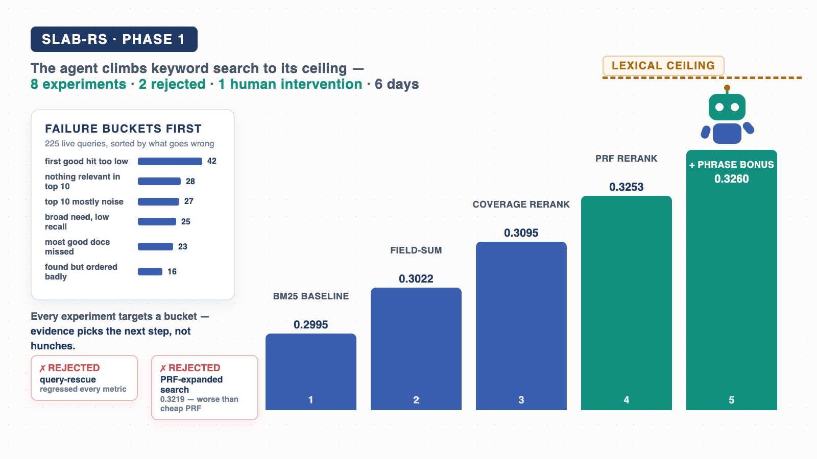
Experiment 1: query-rescue — rejected. The first, most intuitive idea: add bonus scoring for phrase matches and for results that contain every query word, to rescue the worst queries. It made every metric worse. The results stay in the repo as permanent rejected evidence — the first proof the process was honest.
Experiment 2: field-sum — accepted. The boring counterpart won. Instead of scoring a document by its single best field (title or abstract or body), let evidence from all fields add up. nDCG@10: 0.2995 → 0.3022. Small, but everything moved in the right direction.
Experiment 3: coverage-rerank — accepted. Digging into the 28 worst queries showed something useful: for 19 of them, a good document was being found — it was just sitting at rank 11–50 where nobody looks. That is a ranking problem, not a “search can’t find it” problem. So: retrieve the top 50, give a small bonus to results whose title and abstract cover more of the query words, and re-order. nDCG@10 0.3095. But the worst-query count only moved from 28 to 27. The stubborn remainder is a vocabulary problem — the query and its answers use different words entirely. Remember that; it is the cliffhanger.
Experiment 4: pseudo-relevance feedback — the surprise winner. This is a decades-old idea from the IR textbooks (formally: relevance feedback, from the Rocchio lineage). In plain words: assume your top few results are probably decent, look at what words they use, and use those extra words to re-score everything else. The query says “wing pressure distribution”; the top results also talk about “aerofoil” and “spanwise” — so results using those words are probably relevant too.
Here is the part I find genuinely interesting: I have never seen pseudo-relevance feedback actually shipped in a production search system. It usually dies in review for two reasons — a second scoring pass adds latency, and if the top results are bad, the borrowed vocabulary drags the query further off-target.
The agent’s version dodges the latency objection: it reranks inside the already-retrieved top-50 pool. Take the top 4 hits, pull 8 useful words from their titles and abstracts, re-score the pool. No second trip to OpenSearch, no model call, and the explain endpoint shows exactly which words were borrowed. Result: nDCG@10 0.3253 — the biggest single jump of the phase.
Experiment 5a: expanding the search with feedback words — rejected. The obvious next step, actually running a second OpenSearch query with the borrowed words added, made things worse (0.3219). The cheap version of the idea was the right version.
Experiment 5b: a phrase bonus — the last +0.2%. A small tuned bonus for results where the query words appear next to each other as a phrase nudged the score to 0.3260. All of this tuning ran offline against cached result pools, so trying a parameter cost nothing but CPU.
Reality Check Against a Published Paper
This is where my first intervention happened. Watching the numbers climb, I wanted an external yardstick, so I pointed the agent at a published study: Ghasemi and Hiemstra, “BERT meets Cranfield” (EACL 2021), which evaluated BM25 and BERT-based rankers on this same collection. The agent took it from there — it rebuilt the paper’s evaluation conditions on its own so the numbers would be comparable. Matching their setup (binary relevance, their BM25 settings, nDCG@20), our keyword ladder reaches 0.4563, versus their BM25 at 0.4714 and their BERT re-ranker at 0.5525.
Honest position: the keyword ladder closed most of the gap to their BM25, and stayed well below their neural rankers. The gap is quantified, not hand-waved — and it sets up Part 4.
Where the Keyword Road Ends
| Stage | nDCG@10 | vs baseline |
|---|---|---|
| BM25 baseline (released) | 0.2995 | — |
| field-sum | 0.3022 | +0.9% |
| coverage-rerank | 0.3095 | +3.3% |
| pseudo-relevance feedback | 0.3253 | +8.6% |
| + phrase bonus (the ceiling) | 0.3260 | +8.8% |
Look at the increments: each layer bought less than the one before, and the last refinement was worth two tenths of a percent. That is what hitting a ceiling looks like in data. And 27 queries still find nothing relevant in their top 10, because their vocabulary simply does not overlap with the documents that answer them.
Every stage above is live. The explain page runs your query through each architecture side by side and shows the borrowed feedback words and which results the rerank moved.
One more thing worth noticing: the public default search is still the plain baseline. Deliberately. Nothing gets promoted until it proves itself on a second dataset — that is the next phase’s transferability gate. Improving on one benchmark is easy to fake; improving everywhere is the real test. The candidates wait, recorded and reproducible.
The Chain So Far: Eight Experiments, One Human Intervention
Nothing in this article was a random walk — each step was reached from the evidence of the previous one:
- Baseline evaluation (agent) → produced the failure buckets.
- Failure buckets → two targeted candidates: query-rescue (agent, rejected) and field-sum (agent, accepted).
- Drilling into the worst bucket — good docs found but buried at rank 11–50 → coverage-rerank (agent, accepted).
- Coverage-rerank’s leftover failures — results that share too few words with the query → pseudo-relevance feedback (agent, accepted; the big jump).
- PRF’s success → two refinements tested: feedback-expanded search (agent, rejected) and the phrase bonus (agent, accepted).
- My paper pointer → the comparability check against Ghasemi and Hiemstra (built by the agent).
Running total: eight experiments, two rejections, one human intervention. The score went 0.2995 → 0.3260.
Takeaways
- Ship the baseline publicly first — a live, explainable system is the measuring stick that keeps every later claim honest.
- Sort failures into categories before proposing fixes. The categories, not the average, tell you what to build.
- Keep rejected experiments as first-class artifacts — the rejection record is what makes the accepted decisions credible.
- Keyword-based ranking has a ceiling, and you can measure yourself hitting it.
Part 4: what happened when embeddings tried to break that ceiling — including two expensive-looking failures before the breakthrough.